Project Overview
The goal of this assignment is to explore homographies, image warping, and mosaicing. This project demonstrates both manual and automatic approaches to creating panoramic mosaics, with automatic stitching using Harris corner detection, feature matching, and RANSAC for robust homography estimation.
Shoot and Digitize Pictures
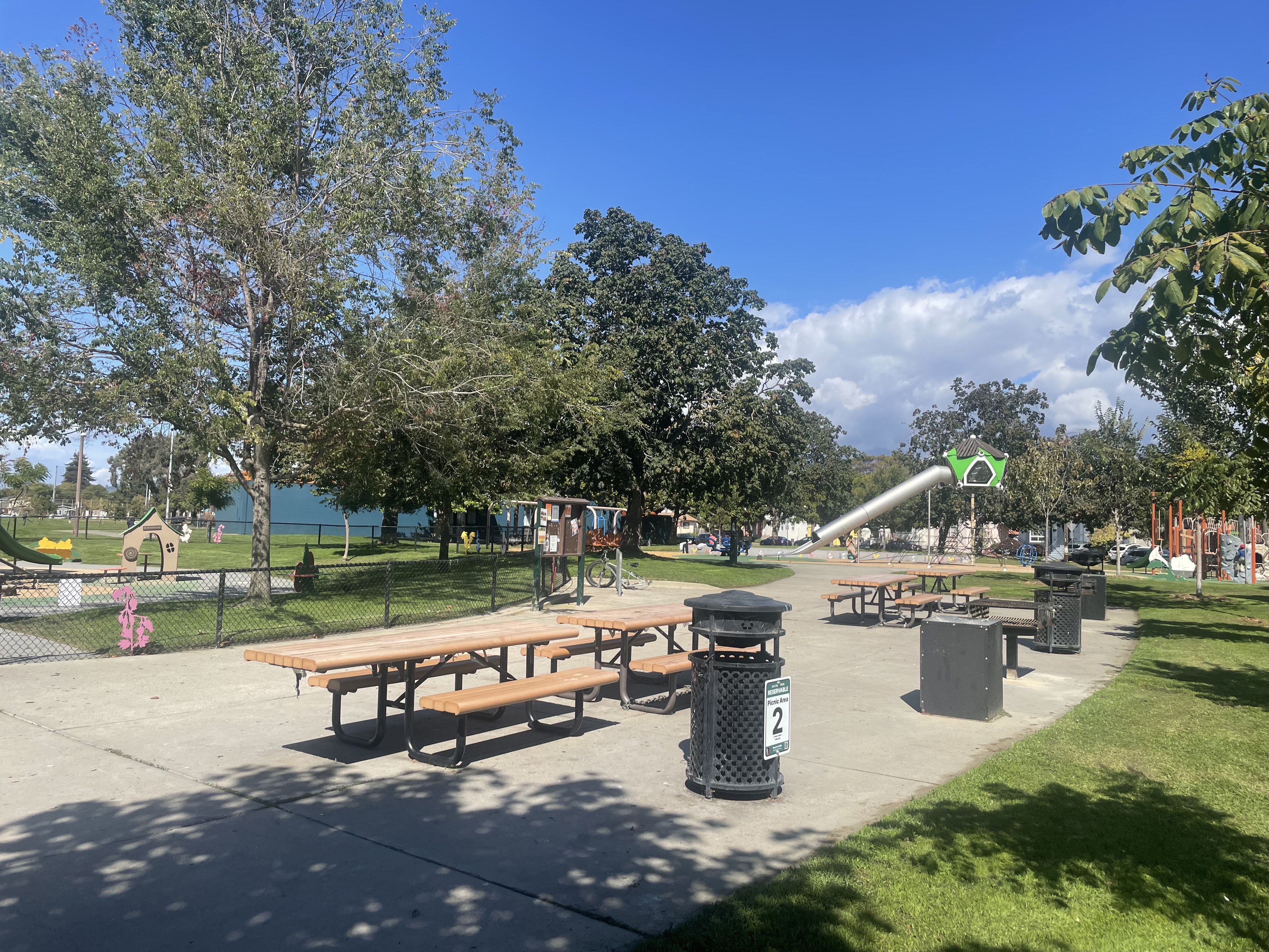
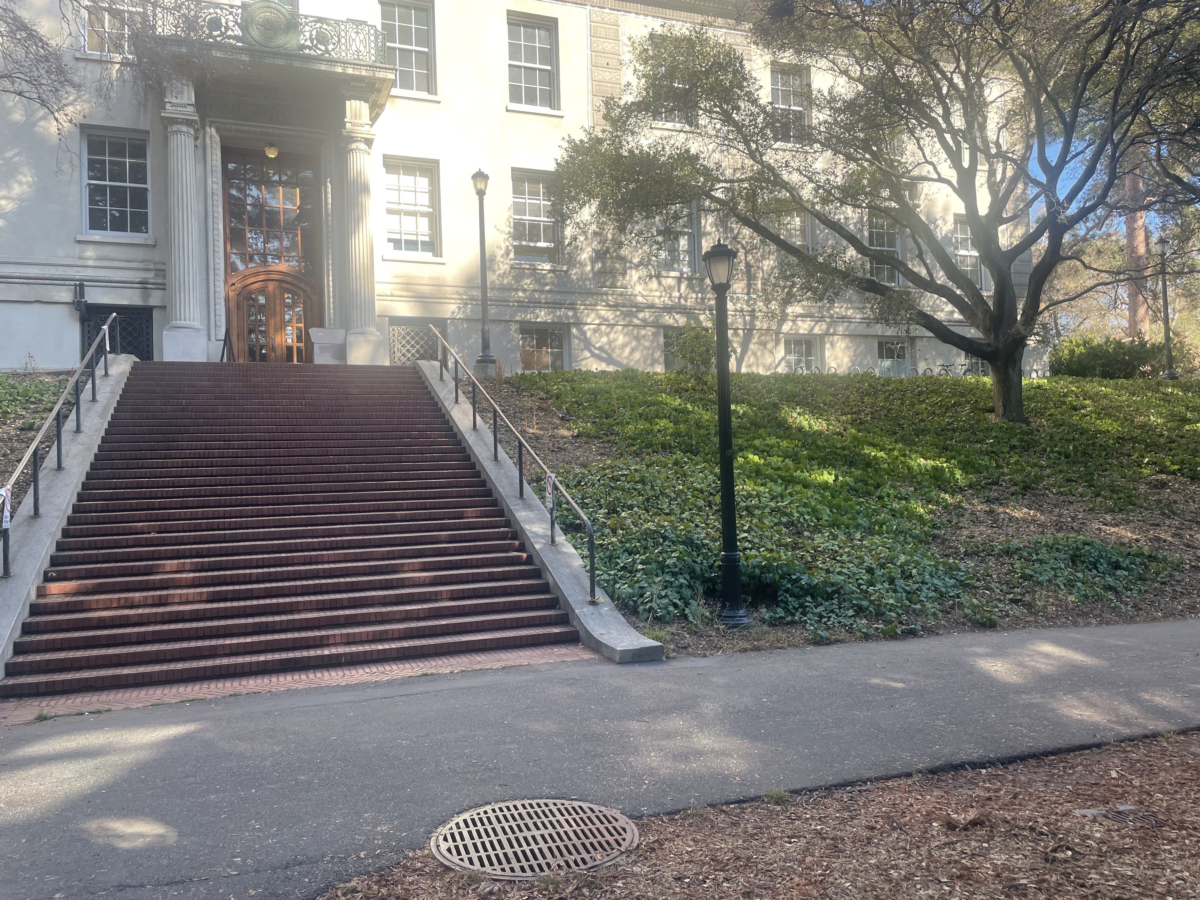
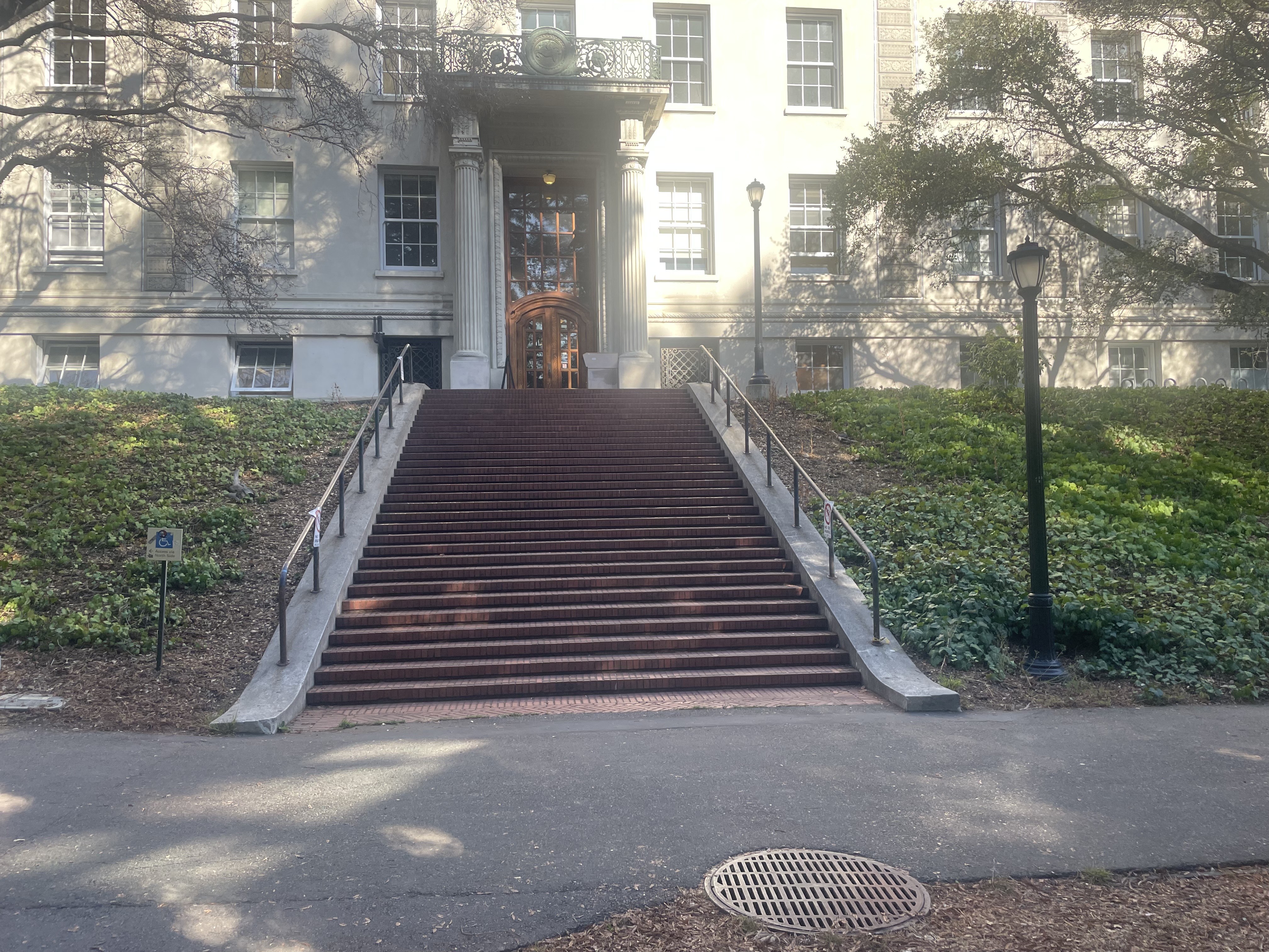
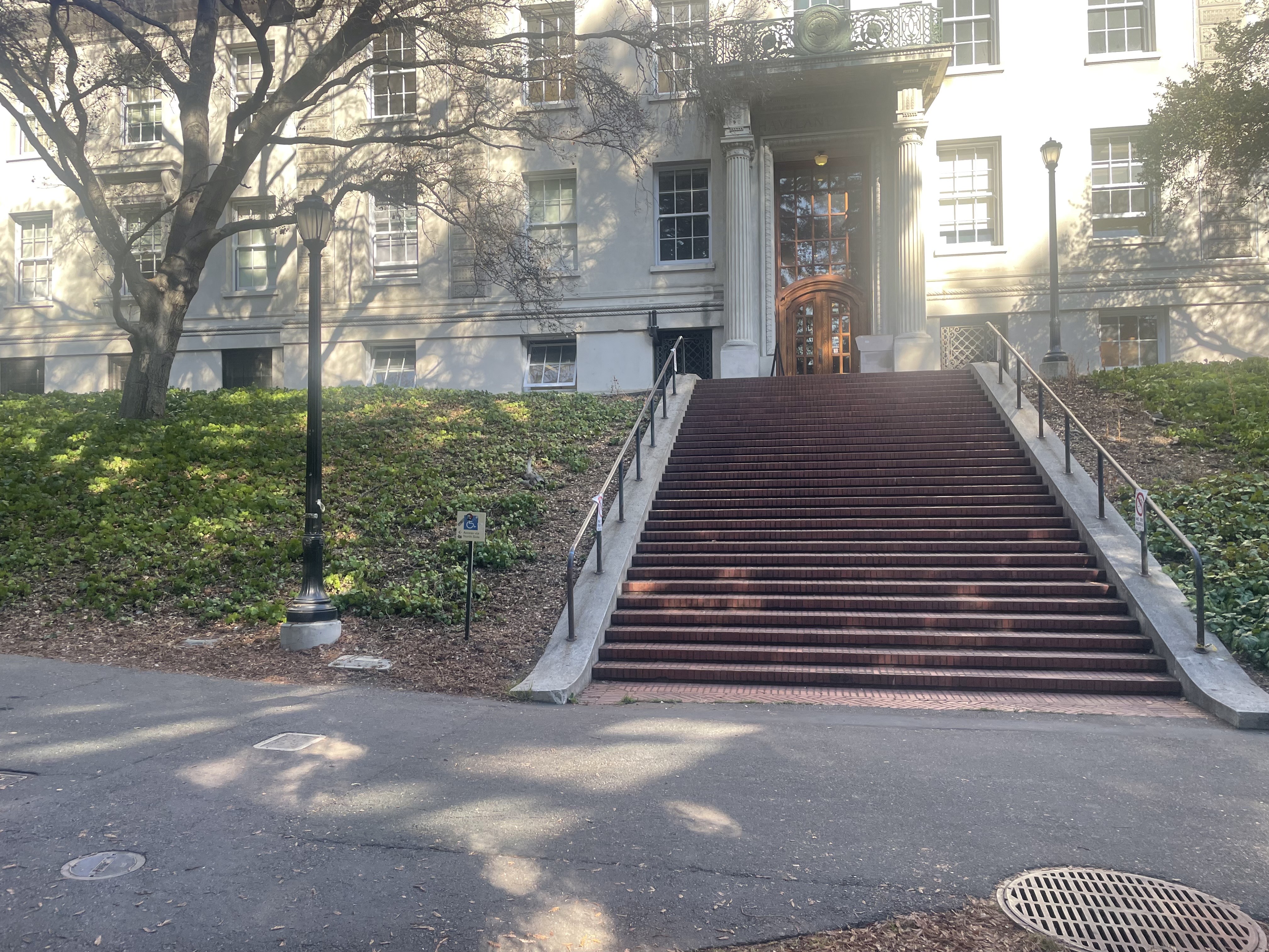
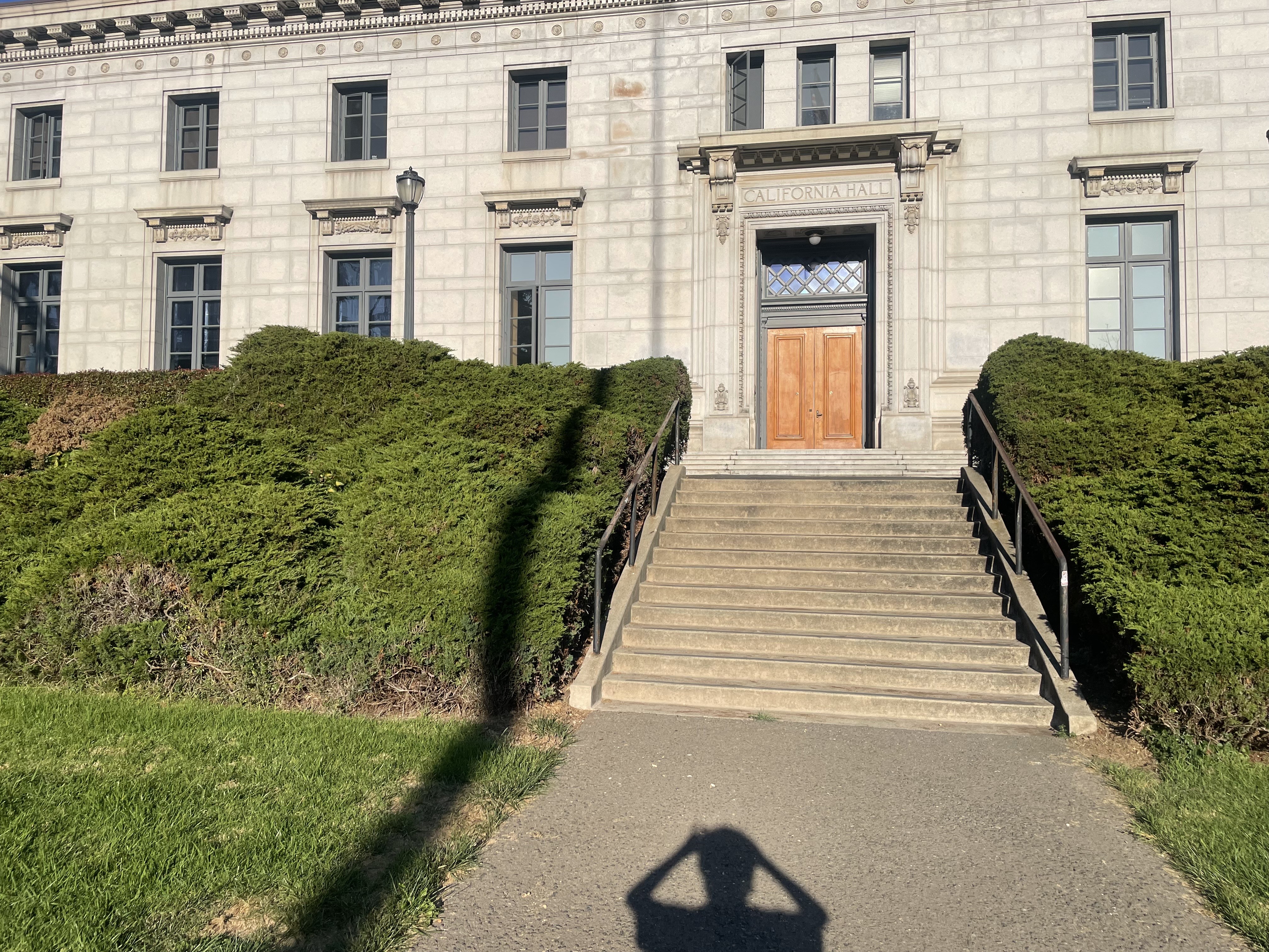
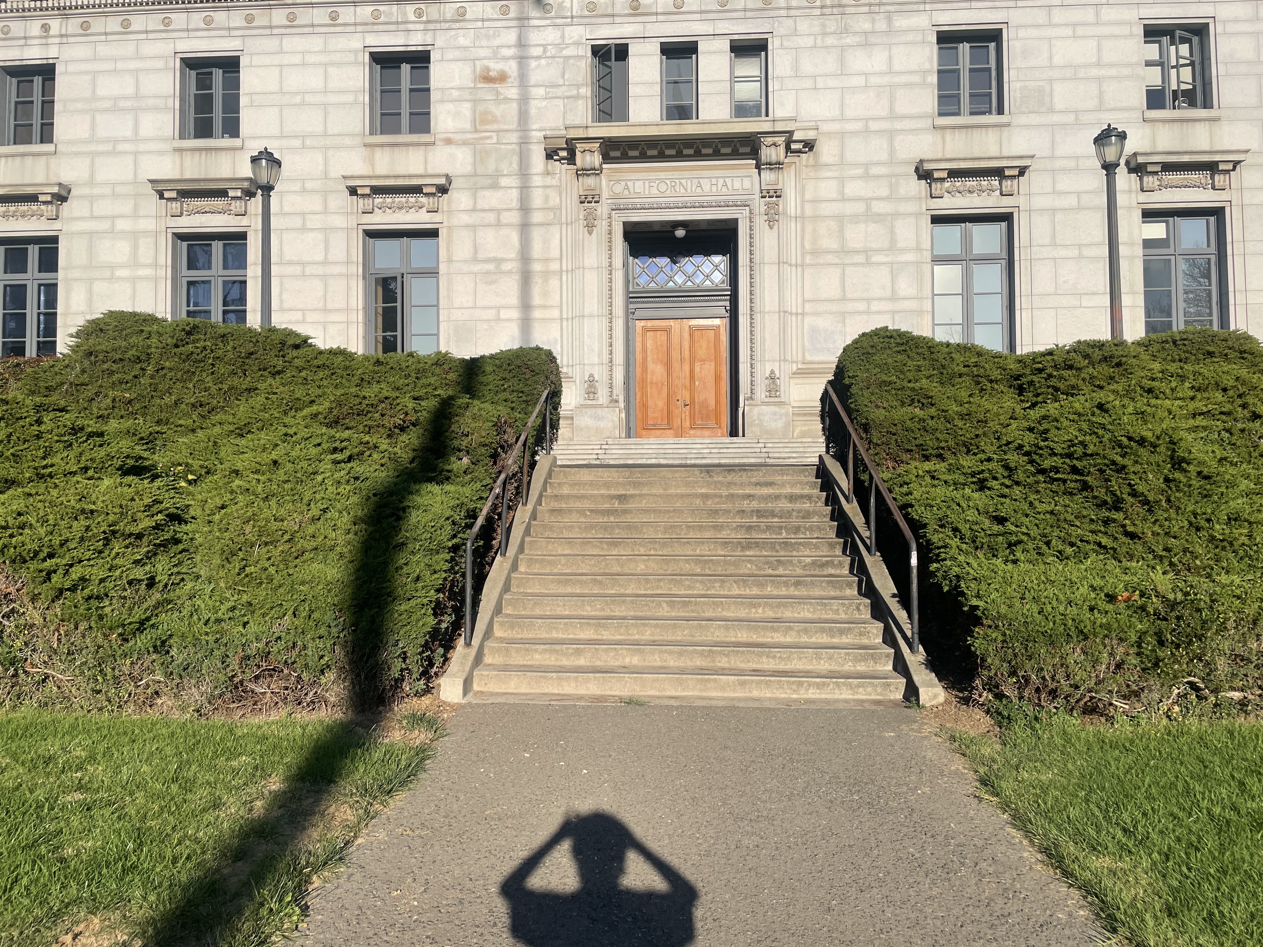
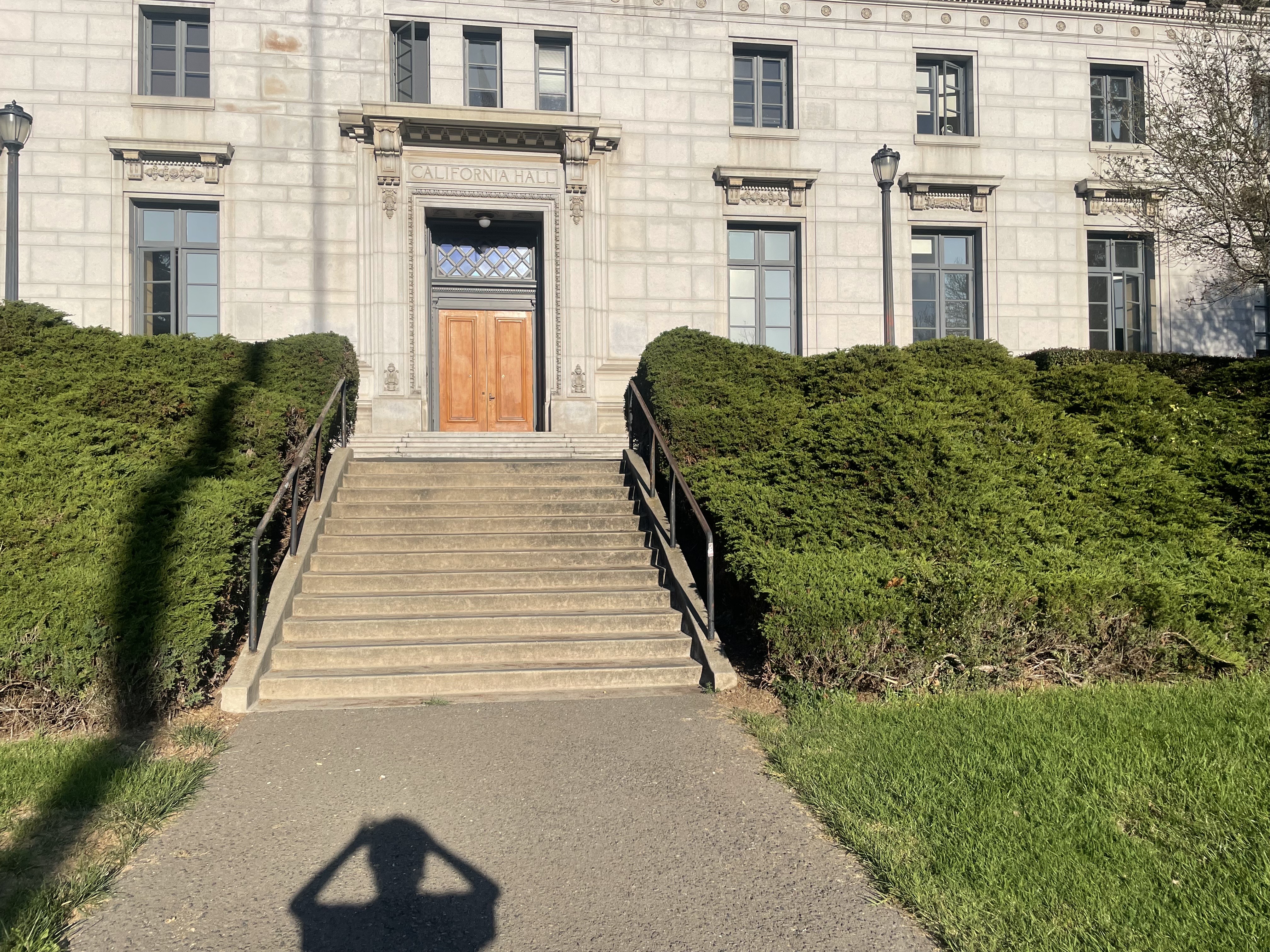
We start by shooting and digitizing pictures of the various scenes we will be using for the final mosaics. The 3 sets I chose was a lovely park by my house, some stairs nearby a building at Berkeley, and the exterior of a building towards the center of campus.
It is critical to take pictures that can be related to eachother via homography. To do this, we need to ensure rays from one picture to the next are captured. This can be enforced by rotating the camera slightly between pictures and never translating the camera's center of projection.
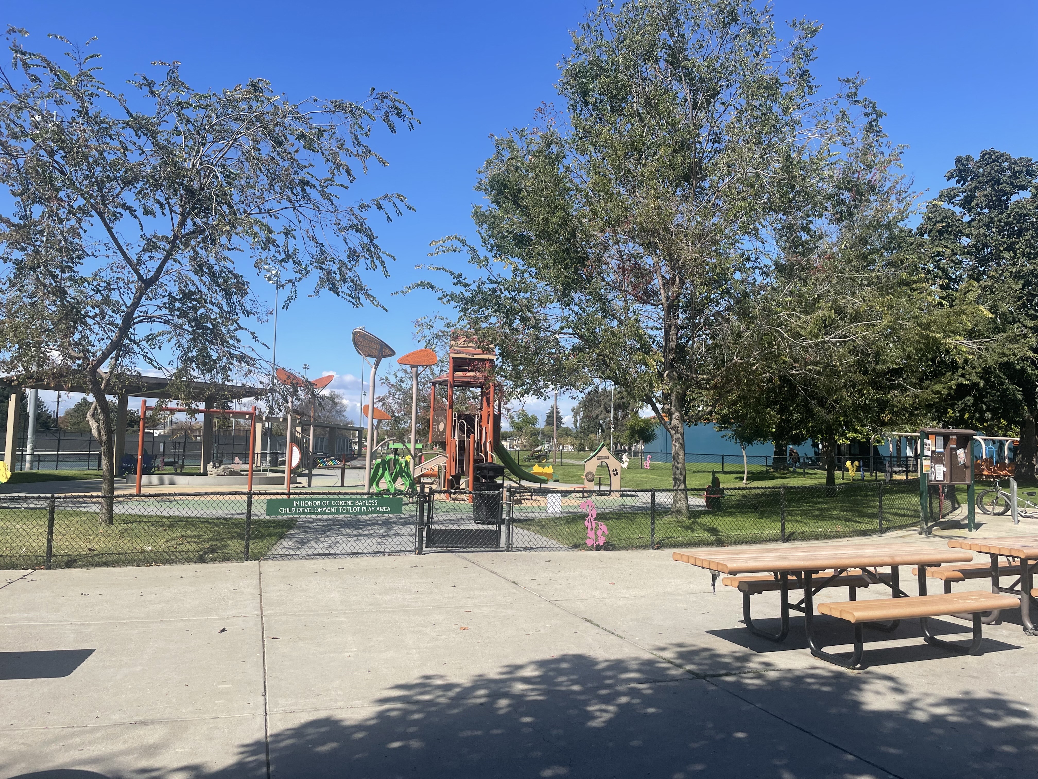
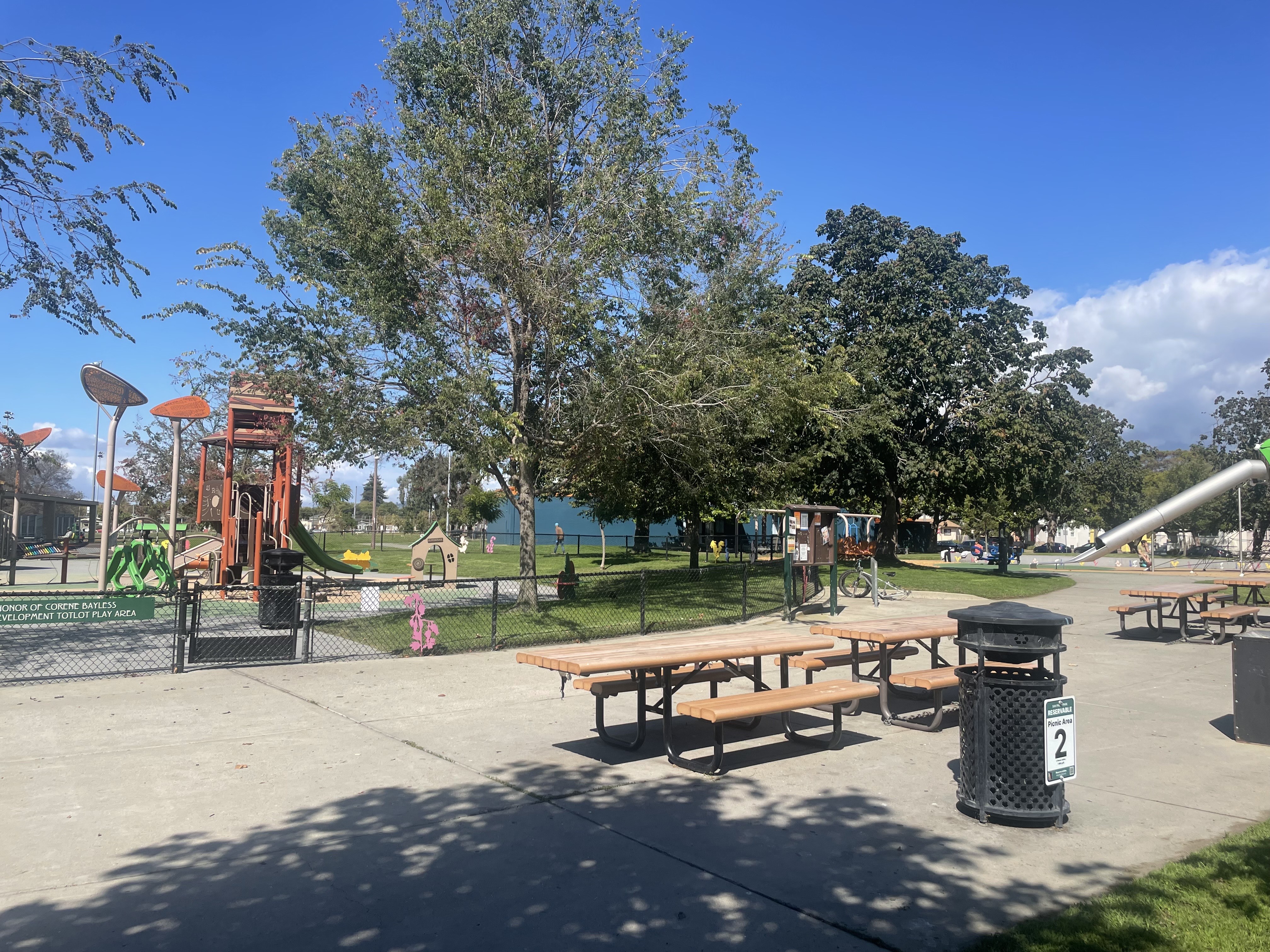
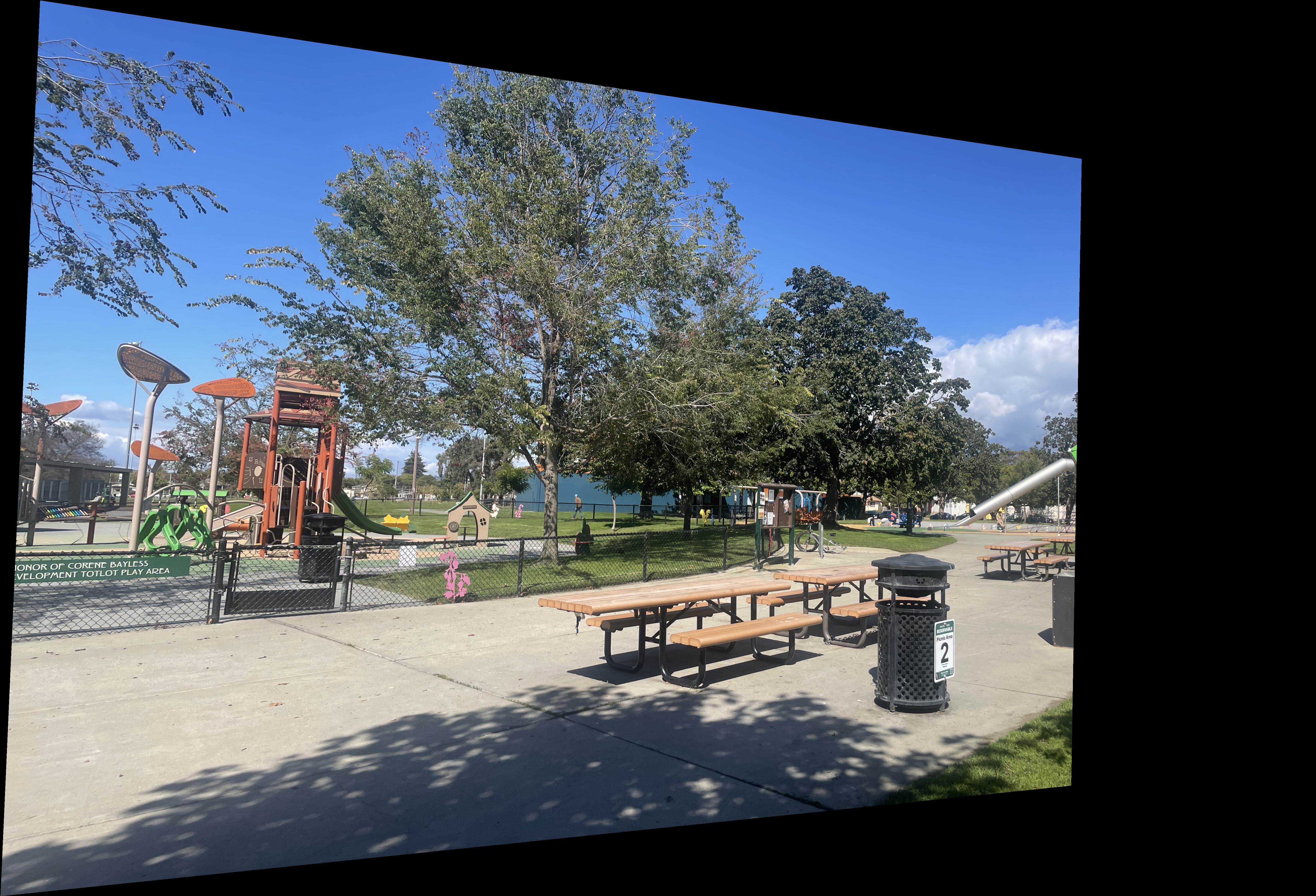
Park Set
Stairs Set
Berkeley Set
Recover Homographies
Now that we have our images, we need to recover the homography transformations between them. We can do this by finding point correspondences between the images (at first manually) and then using the homography matrix to warp the images to a common coordinate system.
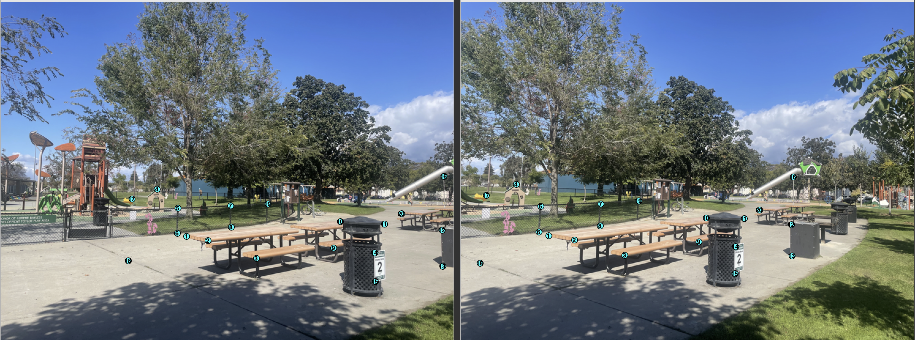
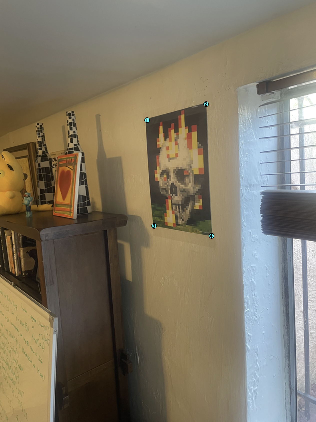
Consider the projective transform relating the second and third picture of the park scene. By manually saving the correspondances between the two images, we can solve an overdetermined system of linear equations to recover the homography matrix. We can see the correspondances visualized below.
Point Correspondences
Mathematical Foundations
Now lets figure out how to mathematically transform our images via a homography so we can use them to create mosaics. A homography is a projective transformation that maps points from one plane to another. For image mosaicing, we need to find the homography matrix that relates corresponding points between two images.
Homography Formulation
For each correspondence $(x,y) \to (u,v)$, the projective transformation gives:
Expanding to linear form and rearranging:
This forms the linear system $\mathbf{D}\mathbf{h} = \mathbf{b}$ where:
With $n$ correspondences, we stack $2n$ equations and solve using least squares to find the 8 unknown homography parameters.
Warped Result
We can now visualize the projective transform between the second and third picture of the park scene. This transform can be applied to any points from the second image using the recovered homography matrix. This gives us a good foundation to start stitching together image mosaics.
Warp the Images (Rectification and Interpolation)
We have figured out how to mathematically recover homography matrices. We can now apply those matrices to images.
Inverse Warping
Instead of forward warping (which can create holes), we use inverse warping. For each pixel $(x', y')$ in the output image, we find the corresponding location $(x, y)$ in the source image:
We then sample the source image at $(x, y)$ using interpolation (nearest neighbor or bilinear) and place that value at $(x', y')$ in the output image. This ensures every output pixel gets a value without holes.
Besides using inverse warping for image mosaics, we can also use it to rectify images since we can use the homography matrix to warp the image to a flat 2D projected rectangle.
Interpolation Tradeoffs
Tradeoffs and Comparisons: Both images appear very similarly across both interpolation methods, however bilinear interpolation is more computationally expesnive resulting in the time it took to generate the image being longer than the nearest neighbor interpolation.
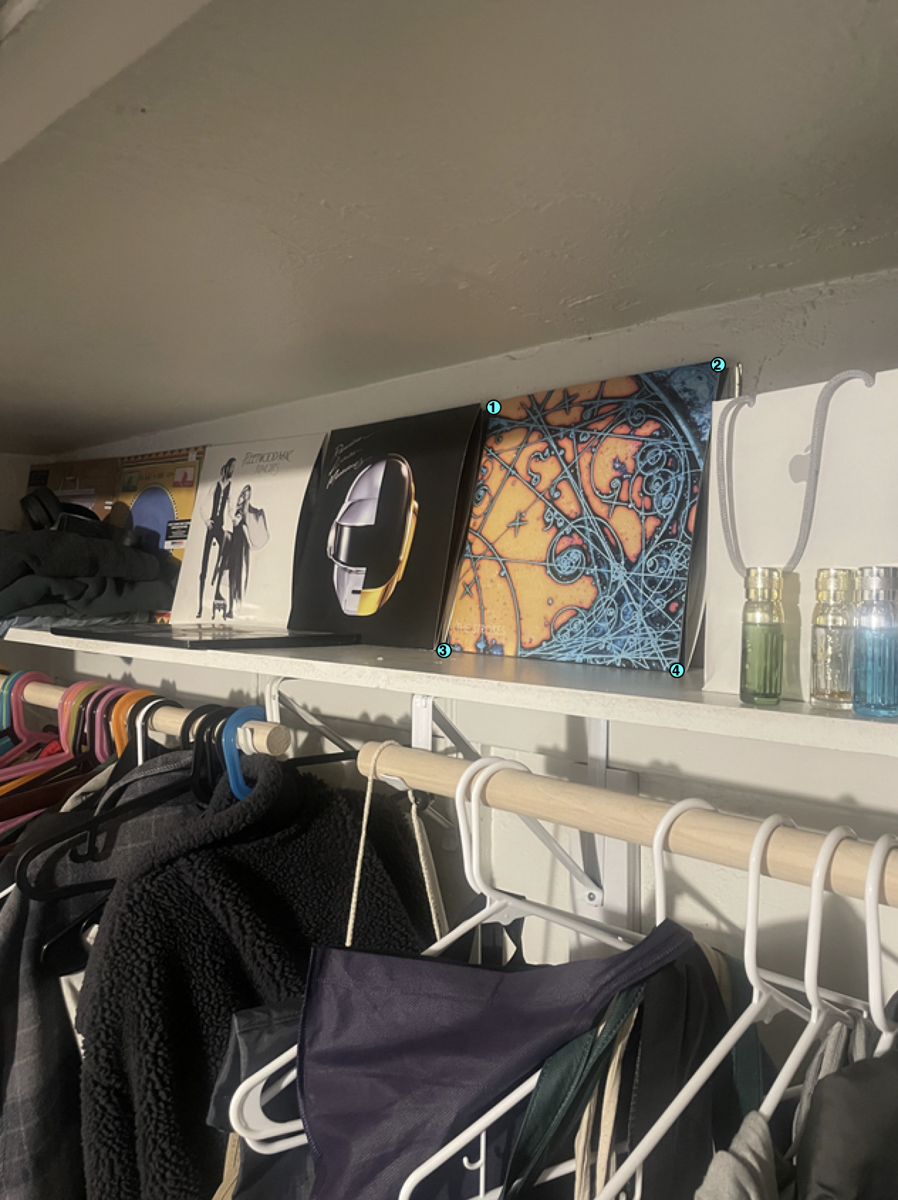
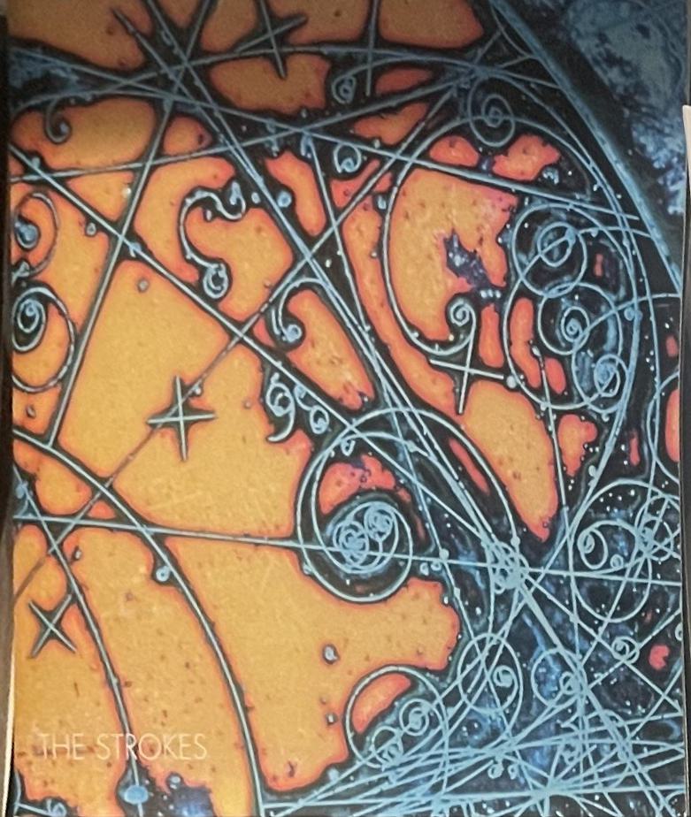
We can visualize more examples of rectification and interpolation below (Recognize any albums?)
Blend Images into a Mosaic
Now for the main event. Using homographies, inverse warping, and interpolation, we can blend our images into beautiful mosaics. To do this, we can learn each homography matrix between an image and a reference image and then use the inverse warping to warp the image to the reference image, apply that homography matrix to each image, then use weighted blending to blend together the images into a single mosaic.
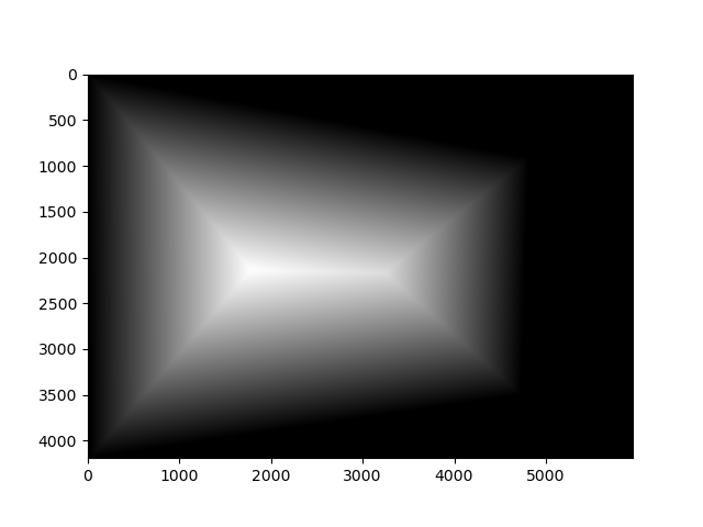
Blending Masks
Below are the masks used for weighted averaging to reduce edge artifacts in the final mosaics. These were generated with scipy.ndimage.distance_transform_edt and allow us to blend
smooth gradients between the images for one final result. Here we can visualize the first source image blended with the center reference image for the park set.

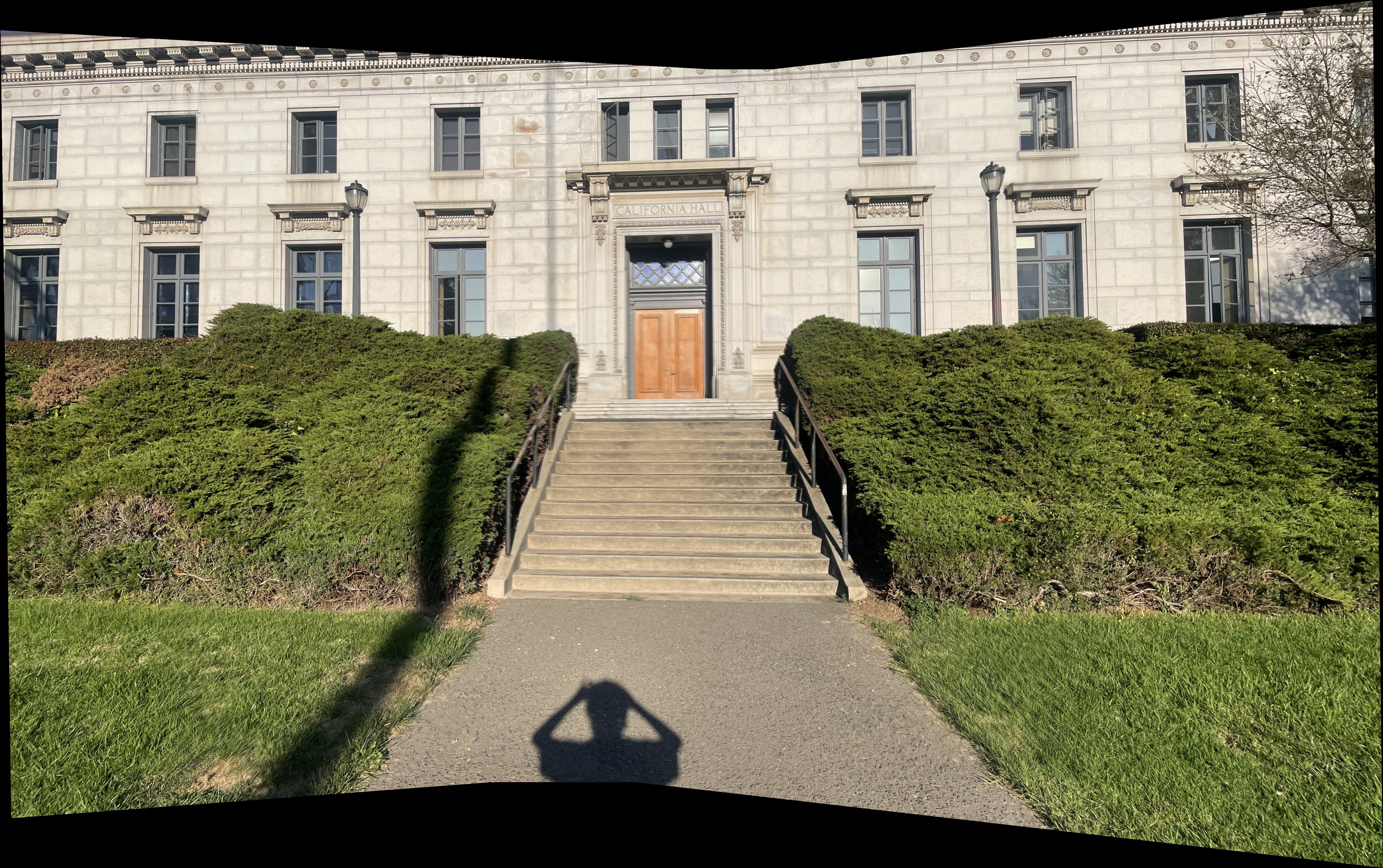
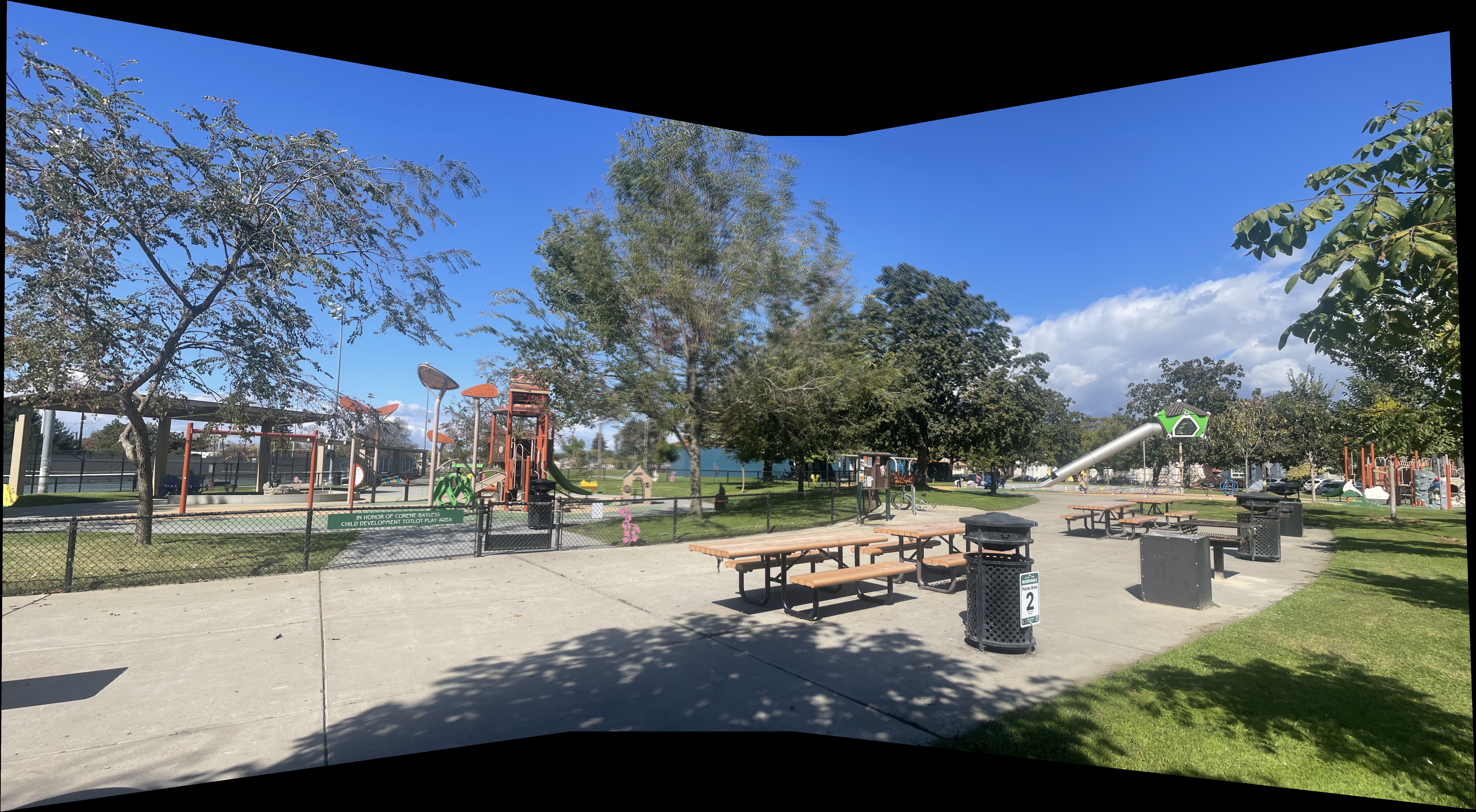
Using these blending masks and everything we learned so far, we can finally visualize our final mosaics! Pay attention to any edge artifacts or blurring especially in the Berkeley Mosaic. These will be reduced when we implement feature detection and autostitching in the next section.
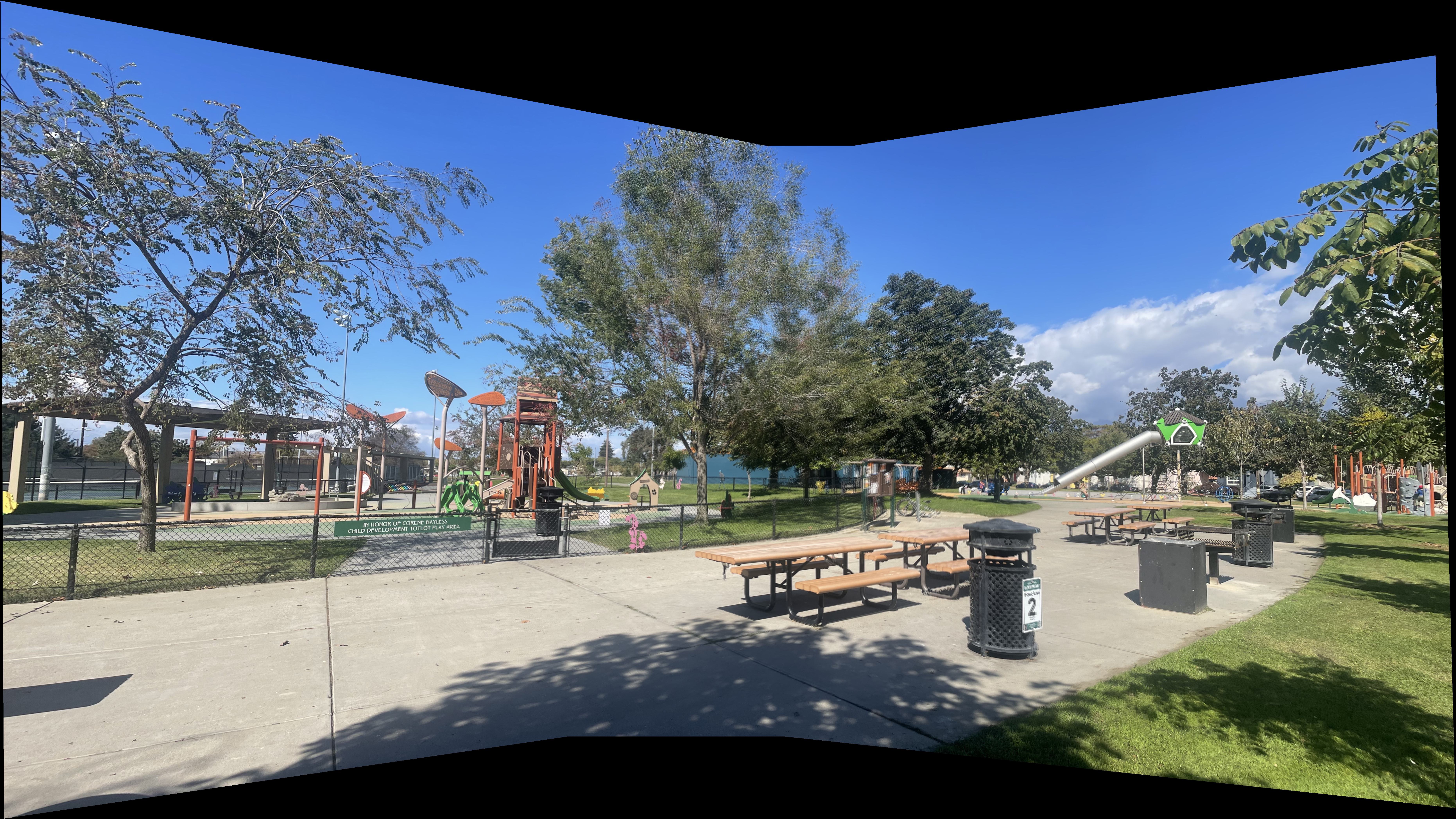
Park Mosaic
Stairs Mosaic

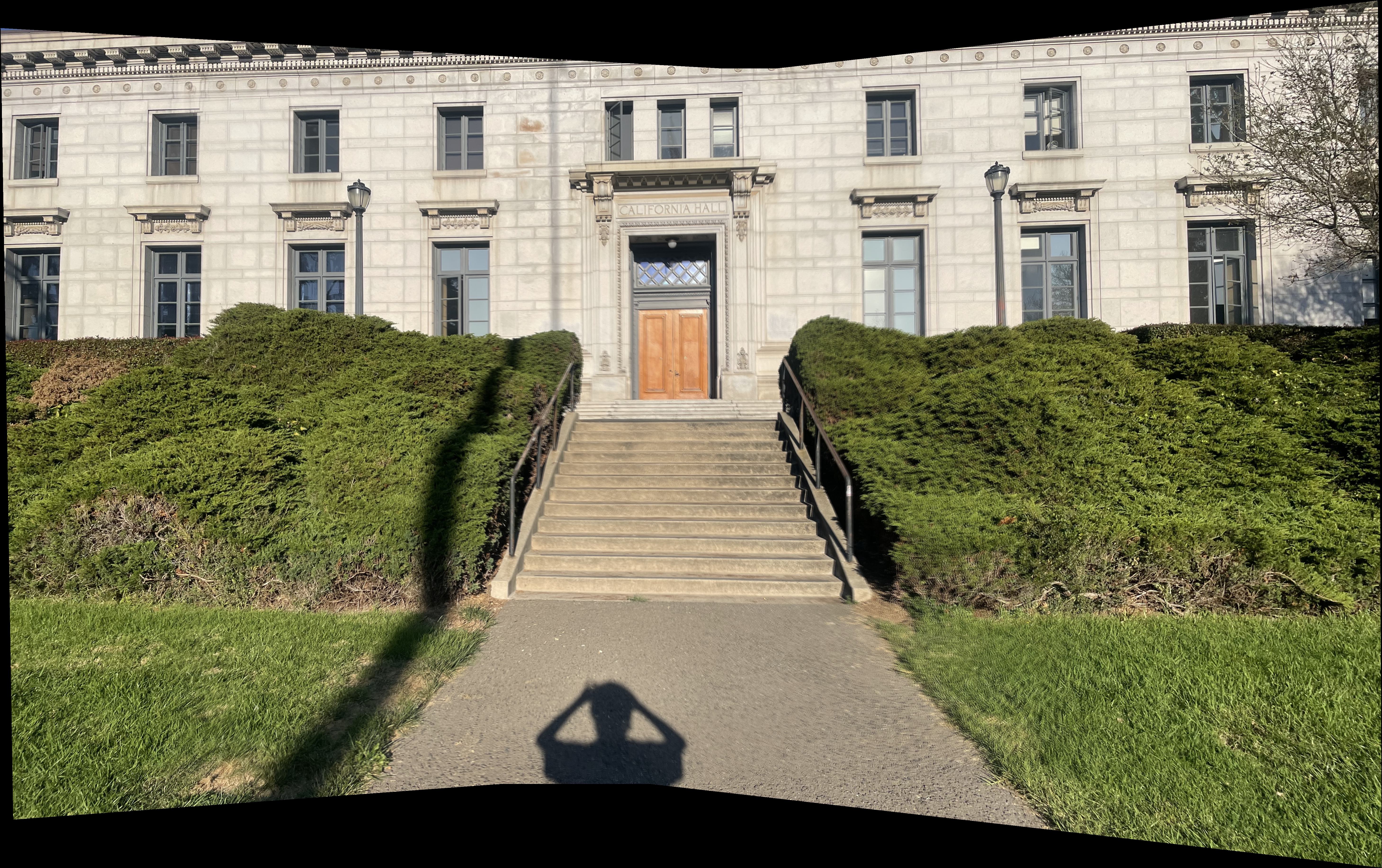
Berkeley Mosaic
We saw how we can create image mosaics using manual correspondances between images. However, this is not always practical and is prone to errors as we saw above. For this next part of the project, we will implement methods to automatically detect features in images and autostitch our images together.
The following parts of this project follows the methodology described in "Multi-Image Matching using Multi-Scale Oriented Patches" by Brown et al. The paper presents a comprehensive approach to automatic image stitching that includes Harris corner detection, adaptive non-maximal suppression, feature descriptor extraction, and robust matching techniques. Note that we do not implement the full framework (such as using wavelet transforms) but nonoftheless the core framework provides the foundation for our automatic mosaicing system.
Harris Corner Detection
The Harris corner detector identifies points of interest in images by analyzing local intensity changes. These corners are characterized by significant intensity variations in multiple directions, making them robust features for image matching.
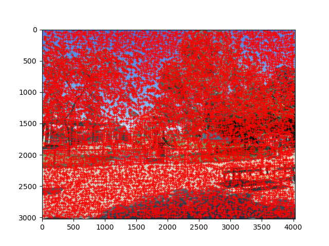
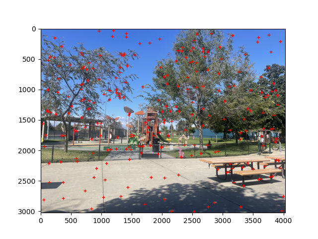
While Harris corner detection is a good starting point, even with a slight bit of filtering it produces a great deal of corners. We can see the effecg of basic Harris corner detection on the first image of the park scene below.
Basic Harris Corner Detection
Adaptive Non-Maximal Suppression (ANMS)
Lets work on optimizing the corners we select. ANMS reduces the number of detected corners while ensuring they are well-distributed across the image. This prevents clustering of corners in high-texture regions and maintains spatial diversity. Below I highlight the effect of ANMS on the above image by filtering down to 250 corners versus 125 corners. Note the fact that corners stay relatively uniformly distributed across the image.

We have successfully found a way to automatically detect a good set of corners for our images. We now need to work on implementing a method to match these corners between images.
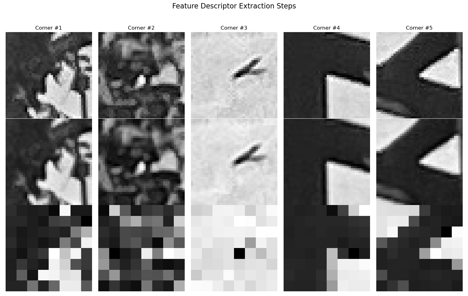
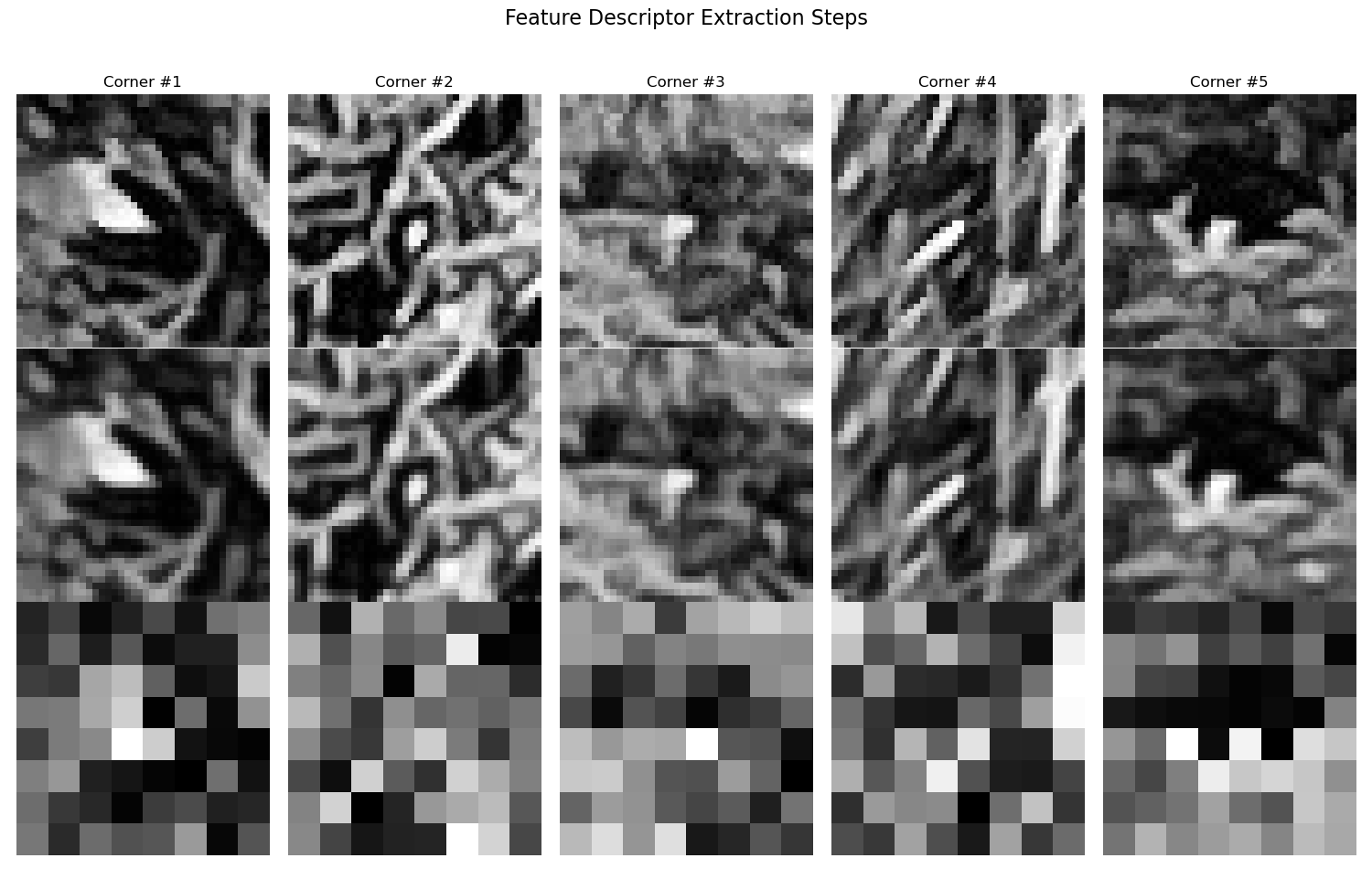
Feature Descriptor Extraction
Feature descriptors capture the local appearance around each detected corner point. With good feature descriptors, it will become significantly easier to match correspondances between images. For this project, 8x8 patches are extracted from a larger 40x40 window, which are then bias/gain-normalized to create robust, illumination-invariant descriptors. Here are some example feature descriptors extracted from the first image of the park scene and the first image of the Berkeley scene.
The first row is the original 40x40 patch, the second row is the blurred 40x40 patch, and the third row is the 8x8 descriptor patch.
Extracted Feature Descriptors
Feature Matching
With good feature descriptors, we can now match correspodances between images. To accomplish this we use the ratio test (Lowe's method) to filter matches based on the ratio between the first and second nearest neighbors, which helps eliminate ambiguous matches.
Lowe's Ratio Test
For each descriptor in image 1, we find its two nearest neighbors in image 2 using Euclidean distance:
where $\mathbf{d}_1^{(i)}$ is the $i$-th descriptor in image 1, and $j_1$ is the index of the first nearest neighbor.
The ratio test accepts a match if:
where $\tau$ is typically 0.7. This ensures the best match is significantly better than the second-best match, reducing false correspondences.
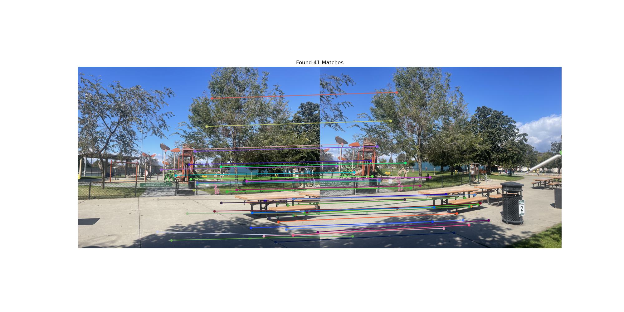
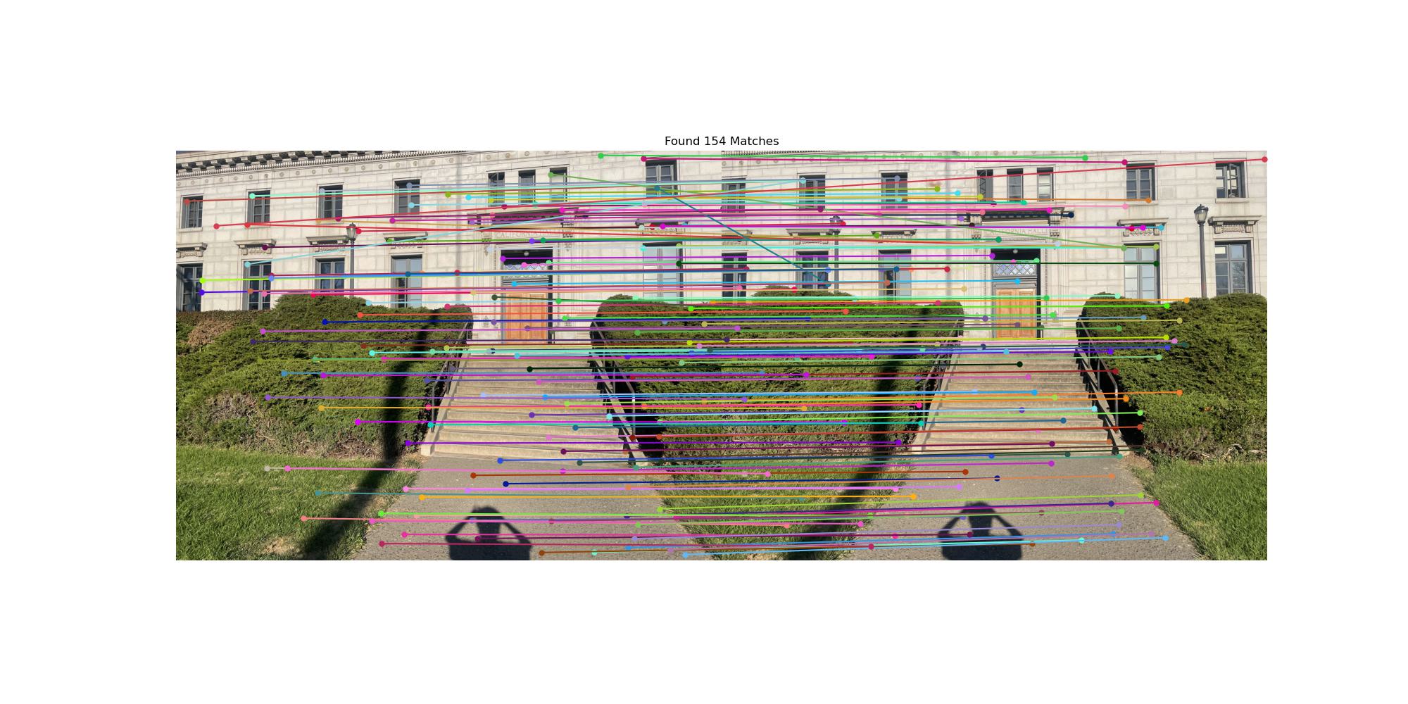
Using Lowe's ratio test, we can now visualize feature matches between a pair of images. Below are the feature matches between the first image of the park scene and the second image of the park scene, and the first image of the Berkeley scene and the second image of the Berkeley scene. Note that there are a significant number of outliers in the Berkeley image due to the repetitive architectural features like windows and building facades that create many similar-looking corners. We can reduce these using RANSAC in the next step.
Feature Correspondences
RANSAC for Robust Homography
We have good feature dsecriptors, we have found a way to match them, but now there are too many outliers that will hurt our homography estimation. By using RANSAC (Random Sample Consensus) we can robustly estimate homographies by iteratively selecting random subsets of correspondences and finding the transformation that best fits the majority of points. This effectively filters out outlier matches and produces more accurate mosaics.
Manual vs Automatic Mosaics
Below are comparisons between manually stitched mosaics (using hand-selected correspondences) and automatically stitched mosaics (using RANSAC-filtered correspondences). The automatic approach demonstrates the robustness of the feature matching and RANSAC pipeline.
Park Mosaic
Stairs Mosaic
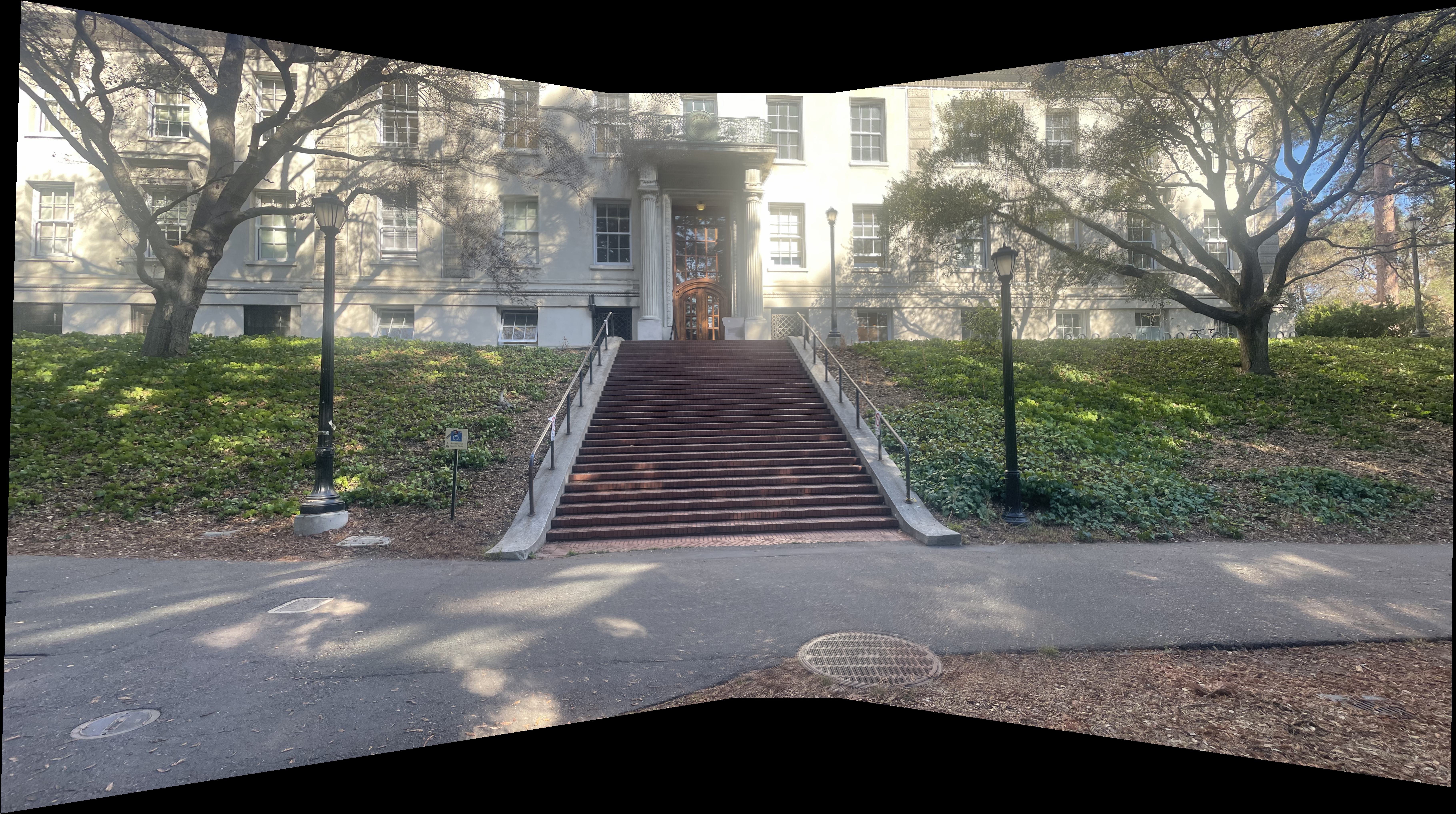
Berkeley Mosaic