


Project Overview
In Part A, we explore pre-trained diffusion models (DeepFloyd IF) to implement sampling loops, denoising techniques, and creative applications like inpainting and optical illusions. This part focuses on understanding how diffusion models work through hands-on experimentation with a state-of-the-art text-to-image model.
Key Concepts
- Forward Process: Adding noise to images progressively
- Denoising: Removing noise using trained UNet models
- Sampling: Generating images from pure noise
- Classifier-Free Guidance (CFG): Improving generation quality
- Image-to-Image: Editing existing images via SDEdit
- Inpainting: Filling masked regions with new content
- Visual Anagrams: Images that change when flipped
- Hybrid Images: Combining low/high frequencies from different prompts
Fun with Diffusion Models
Part 0: Setup and Text Prompts
We use the DeepFloyd IF diffusion model, a two-stage model that generates 64×64 images in the first stage and upsamples them to 256×256 in the second stage. After setting up access to DeepFloyd and generating prompt embeddings, we experiment with custom text prompts.
Setup Notes
- Model: DeepFloyd/IF-I-XL-v1.0 from Hugging Face
- Prompt embeddings generated via Hugging Face clusters
- Random seed used consistently throughout: 777
Custom Text Prompts
I created several interesting text prompts and generated their embeddings. Here are 3 examples with their generated images at different inference steps:
20 Inference Steps
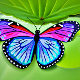
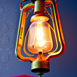
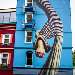
100 Inference Steps
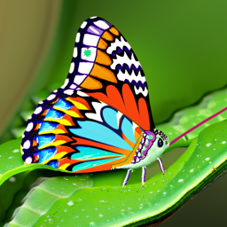
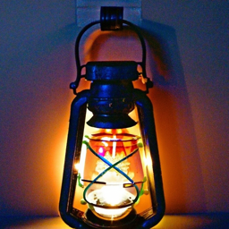
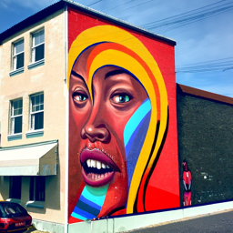
Reflection: The generated images show good alignment with their text prompts. The butterfly prompt produces detailed wing patterns, the lantern captures the light emission effect, and the mural displays building-side artwork. Increasing inference steps from 20 to 100 improves image quality and detail, with 100 steps producing sharper, more coherent results. However, the improvement is incremental, suggesting diminishing returns beyond a certain number of steps.
Part 1.1: Implementing the Forward Process
The forward process takes a clean image $x_0$ and adds noise to it at timestep $t$, producing a noisy image $x_t$. This is defined by:
where $\epsilon \sim \mathcal{N}(0, I)$ is random noise and $\bar{\alpha}_t$ controls the noise level. We test this on the Berkeley Campanile image at different noise levels.


Part 1.2: Classical Denoising
Before using the diffusion model, we attempt to denoise the images using classical Gaussian blur filtering. This serves as a baseline to compare against the learned denoising capabilities of the diffusion model.
Noisy Images (Forward Process)
Classical Denoising (Gaussian Blur)


As expected, classical Gaussian blur filtering struggles to remove noise effectively, especially at higher noise levels. The diffusion model will show significantly better results.
Part 1.3: One-Step Denoising
Now we use the pretrained UNet to denoise images. The UNet predicts the noise in a noisy image, which we can then remove to recover an estimate of the original image. This demonstrates the model's ability to project noisy images back onto the natural image manifold.
Noisy Images (Forward Process)
One-Step Denoised


The UNet does a much better job than Gaussian blur, successfully projecting images back onto the natural image manifold. However, quality degrades with more noise, which motivates iterative denoising.
Part 1.4: Iterative Denoising
Instead of denoising in a single step, we implement iterative denoising by taking multiple steps through the diffusion process. We use strided timesteps (starting at 990, stride of 30) to speed up the process while maintaining quality. The iterative denoising formula is:
Mathematical Foundation of Iterative Denoising
The formula for iterative denoising from timestep $t$ to $t'$ (where $t' < t$) is:
where:
- $x_t$ is your image at timestep $t$
- $x_{t'}$ is your noisy image at timestep $t'$ where $t' < t$ (less noisy)
- $\bar{\alpha}_t$ is defined by $\text{alphas\_cumprod}$, as explained above
- $\alpha_t = \frac{\bar{\alpha}_t}{\bar{\alpha}_{t-1}}$
- $\beta_t = 1 - \alpha_t$
- $x_0$ is our current estimate of the clean image using one-step denoising
- $v_{\sigma}$ is random noise, which in the case of DeepFloyd is also predicted. The process to compute this is not very important, so we supply a function, $\text{add\_variance}$, to do this for you.
This formula allows us to iteratively denoise an image by moving from noisier timesteps ($t$) to less noisy timesteps ($t'$), effectively interpolating between the noisy signal and the clean image estimate.


Iterative denoising produces the best results, gradually refining the image through multiple steps. One-step denoising struggles with high noise levels, and Gaussian blur is clearly inferior.
Part 1.5: Diffusion Model Sampling
We can generate images from scratch by starting with pure noise and iteratively denoising it. This demonstrates the generative capabilities of the diffusion model.
Here are 5 sampled images using the prompt "a high quality photo":


The generated images show reasonable quality but could be improved. We'll use Classifier-Free Guidance (CFG) in the next section to enhance quality.
Part 1.6: Classifier-Free Guidance (CFG)
Classifier-Free Guidance improves image quality by combining conditional and unconditional noise estimates. The formula is:
where $\gamma > 1$ amplifies the effect of the text prompt. We use $\gamma = 7.5$.
Here are 5 images generated with CFG using the prompt "a high quality photo":


The images generated with CFG show significantly improved quality and better alignment with the text prompt compared to unconditional sampling.
Part 1.7: Image-to-Image Translation (SDEdit)
SDEdit allows us to edit existing images by adding noise and then denoising with the diffusion model. The amount of noise added controls how much the image changes. We test this on the Campanile and custom images at different noise levels (i_start = [1, 3, 5, 7, 10, 20]).


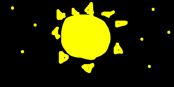
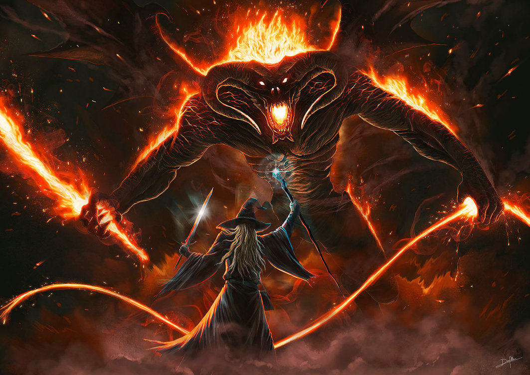
1.7.1: Hand-Drawn and Web Images
SDEdit works particularly well with non-realistic images like sketches or paintings. Here are examples starting from hand-drawn images and web images:


1.7.2: Inpainting
Inpainting allows us to fill masked regions of an image with new content. We use the RePaint algorithm, which preserves unmasked regions while generating new content in masked areas.


1.7.3: Text-Conditional Image-to-Image Translation
By using text prompts during SDEdit, we can guide the image transformation. I am using the prompt "a group of frogs playing in a band" for all the following text-guided edits:


Part 1.8: Visual Anagrams
Visual anagrams create optical illusions where an image looks like one thing when viewed normally, but reveals a different image when flipped upside down. We achieve this by averaging noise estimates from two different prompts—one for the normal orientation and one for the flipped orientation.
where $p_1$ and $p_2$ are two different text prompts, and we average the noise estimates to create the final image.


Part 1.9: Hybrid Images
Hybrid images combine low-frequency information from one prompt with high-frequency information from another, similar to Project 2. We use Gaussian blur to separate frequencies and create composite noise estimates.
where UNet is the diffusion model UNet, $f_{\text{lowpass}}$ is a low pass function, $f_{\text{highpass}}$ is a high pass function, and $p_1$ and $p_2$ are two different text prompt embeddings. Our final noise estimate is $\epsilon$.


Hybrid images showcase the frequency-domain capabilities of diffusion models, allowing us to create images that appear different at different viewing distances or scales.
Building a U-Net
Project Overview
In Part B, we build and train our own flow matching model on MNIST using PyTorch. This involves implementing a UNet architecture from scratch, training it for single-step denoising, and then extending it to iterative flow matching with time and class conditioning.
Key Concepts
- UNet Architecture: Encoder-decoder network with skip connections
- Single-Step Denoising: Training a denoiser to map noisy images to clean images
- Flow Matching: Learning the velocity field to iteratively denoise images
- Time Conditioning: Injecting timestep information into the UNet
- Class Conditioning: Conditioning generation on digit classes (0-9)
- Classifier-Free Guidance: Improving generation quality through guidance
Part 1: Training a Single-Step Denoising UNet
We start by building a simple one-step denoiser. Given a noisy image, we aim to train a denoiser that maps it to a clean image.
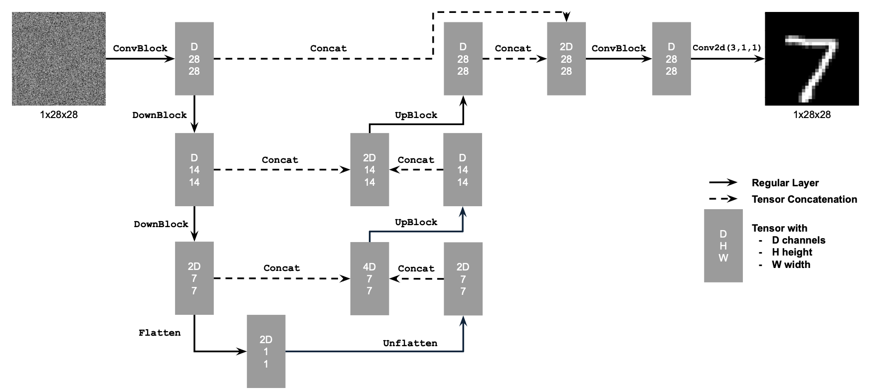
1.1 Implementing the UNet
We implement a denoiser as a UNet that maps noisy images to clean images. The objective loss function for training the denoiser is:
where $D_\theta$ is the denoiser with parameters $\theta$, $z$ is a noisy image, and $x$ is the corresponding clean image. The expectation is taken over the distribution of noisy-clean image pairs.
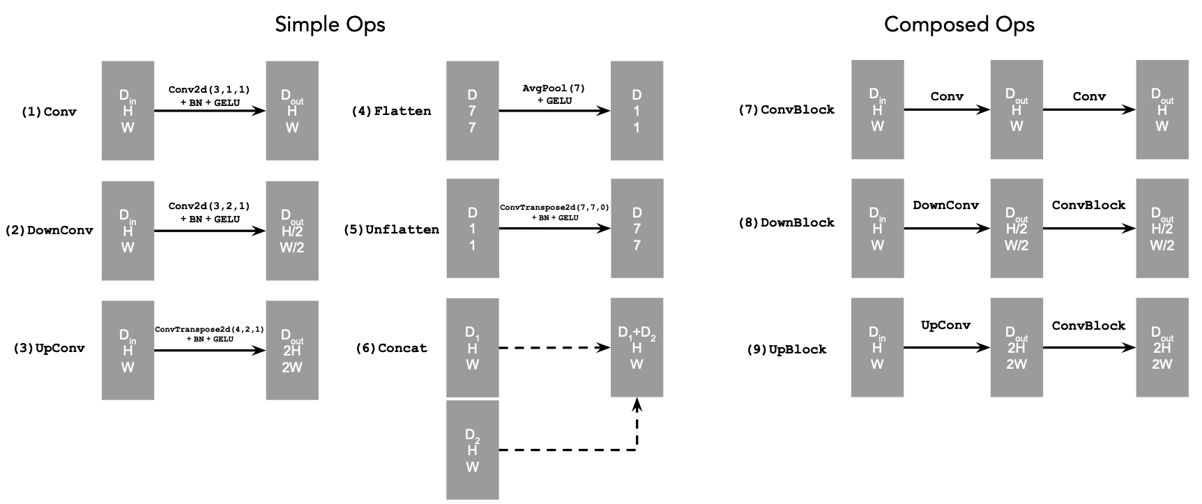
The UNet consists of downsampling and upsampling blocks with skip connections. The architecture uses standard operations like Conv2d, ConvTranspose2d, BatchNorm, GELU activation, and AvgPool2d for flattening/unflattening operations. We use hidden dimension D = 128 for the single-step denoising UNet.
1.2 Using the UNet to Train a Denoiser
Recall from equation 1 that we aim to solve the following denoising problem: Given a noisy image $z$, we aim to train a denoiser $D_\theta$ such that it maps $z$ to a clean image $x$. To do so, we can optimize over an L2 loss:
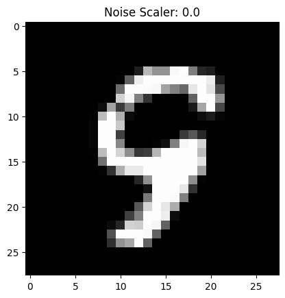
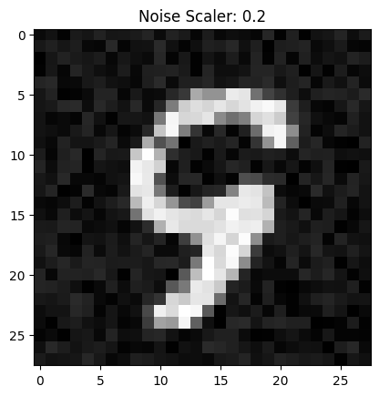
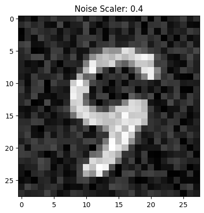
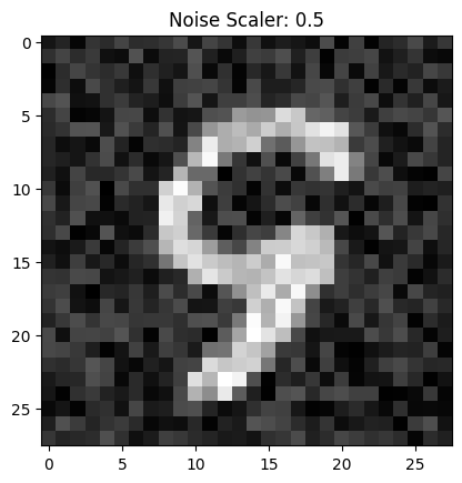
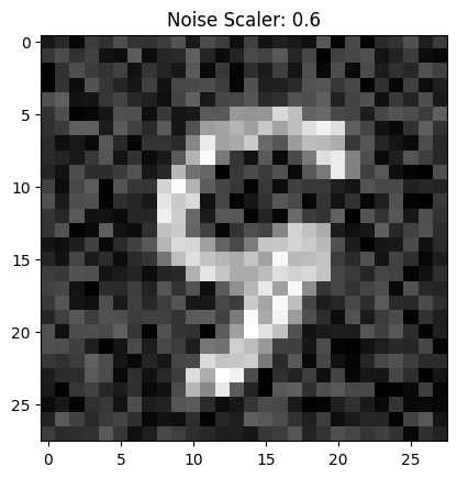
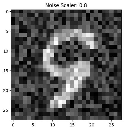
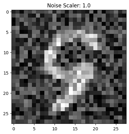
To train our denoiser, we need to generate training data pairs of $(z, x)$, where each $x$ is a clean MNIST digit. For each training batch, we can generate $z$ from $x$ using the following noising process (Forward Process):
where $\sigma$ is a scalar noise level and $\epsilon$ is random noise drawn from a standard normal distribution.
We can visualize the different noising processes over $\sigma \in [0.0, 0.2, 0.4, 0.5, 0.6, 0.8, 1.0]$, assuming normalized $x \in [0, 1]$. Note that images become noisier as $\sigma$ increases.
1.2.1 Training
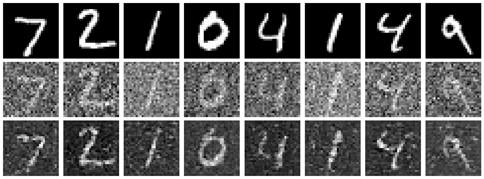
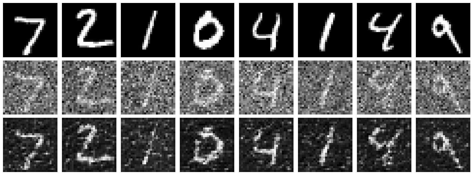
We train the model on the MNIST training set with a batch size of 256 for 5 epochs. The model uses a UNet with hidden dimension D = 128, Adam optimizer with learning rate 1e-4, and noise level $\sigma = 0.5$.
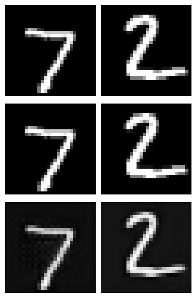
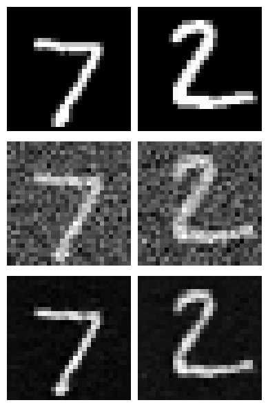
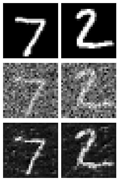
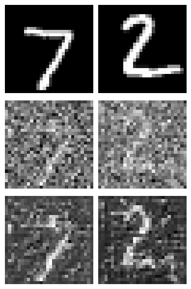
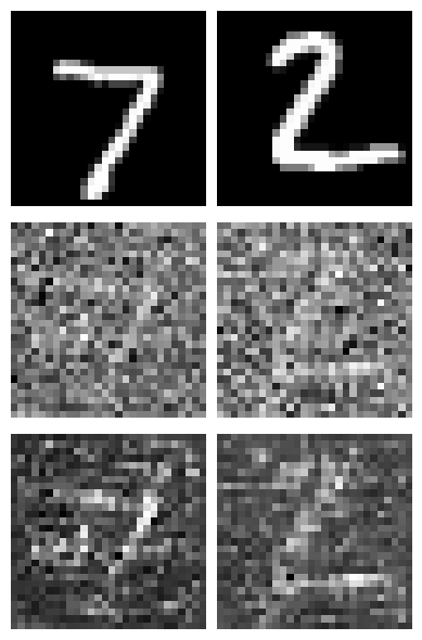
Lets sample some results on the test set with noise level 0.5 after the first and the 5th epoch. Each image shows three rows: the original image (top), the noisy image with added noise (middle), and the denoised result (bottom). Clearly the model improves as training goes on but its important to note this model is trained only on one noise level (0.5) and may not generalize well to other noise levels.
1.2.2 Out-of-Distribution Testing
Our denoiser was trained on MNIST digits noised with $\sigma = 0.5$. Let's see how it performs on different $\sigma$ values that it wasn't trained for.
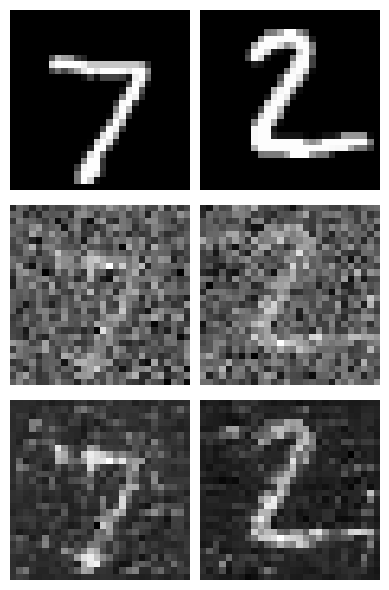
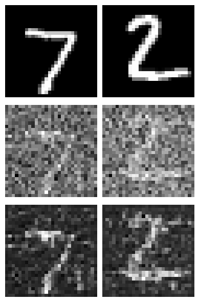
Clearly the model performs poorly on out-of-distribution noise levels especially at higher noise levels. This is expected as the model was trained only on one noise level (0.5).
1.2.3 Denoising Pure Noise
We now transition to making denoising a generative task. We train the model to denoise pure, random Gaussian noise. We can think of this as starting with a blank canvas $x_\sigma$ where $\sigma = 1$ and denoising it to get a clean image $x_0$. Once again we can display testing samples after the first and the 5th epoch to gauge model performance.
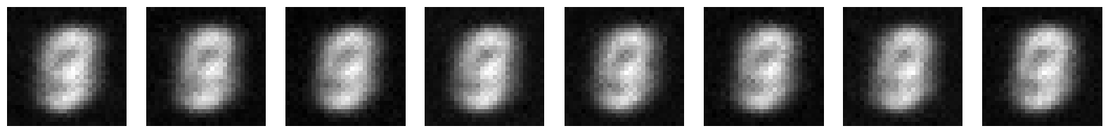
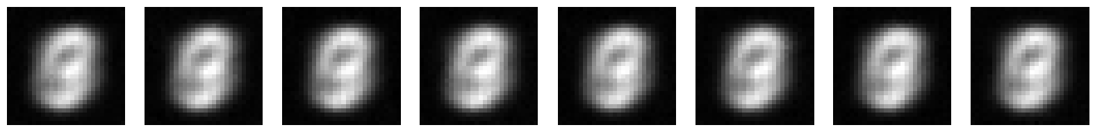
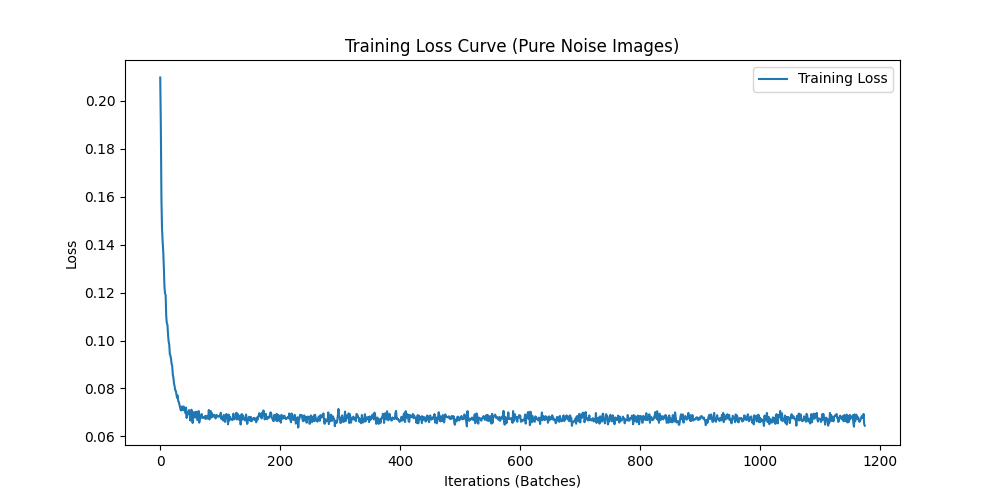
Key Observation
The generated outputs show blurry, averaged representations of digits. With an MSE loss, the model learns to predict the point that minimizes the sum of squared distances to all training examples—essentially the centroid of the digit distribution. This results in outputs that look like averaged versions of all digits rather than distinct digit samples.
Part 2: Training a Flow Matching Model
One-step denoising does not work well for generative tasks. Instead, we need to iteratively denoise the image using flow matching. We train a UNet model to predict the 'flow' from noisy data to clean data.
For iterative denoising, we define intermediate noisy samples using linear interpolation between noisy $x_1$ and clean $x_0$. The flow matching formulation is as follows:
Mathematical Foundation of Flow Matching
For iterative denoising, we define intermediate samples and the flow:
where:
- $x_0$ is a clean image sampled from distribution $p_0(x_0)$
- $x_1$ is a noisy image sampled from distribution $p_1(x_1)$
- $t \in [0, 1]$ is a timestep sampled uniformly from $U_{[0,1]}$
- $x_t$ is the interpolated sample at timestep $t$
- $u(x_t, t)$ is the true flow (velocity) from $x_t$ to $x_0$
Our aim is to learn a UNet $u_\theta(x_t, t)$ which approximates this flow, giving us our learning objective:
We can think of this as training a Unet to solve a ODE problem where the velocity field is given by $u(x_t, t) = x_1 - x_0$. When we have that learned velocity field, we can use it to iteratively denoise the image by solving the ODE backwards in time.
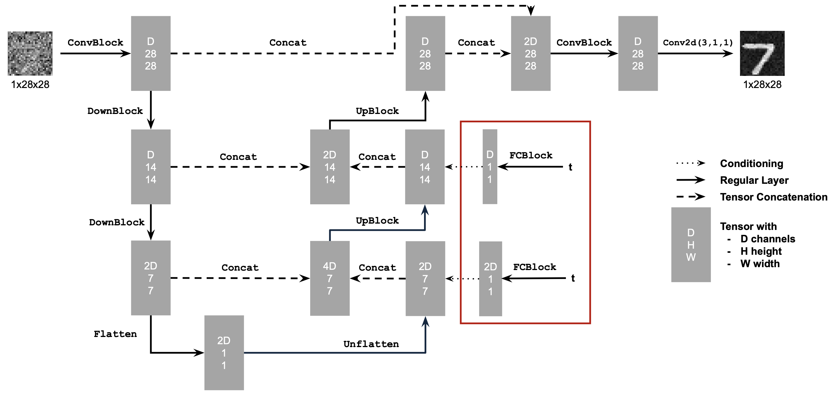
2.1 Adding Time Conditioning to UNet
To model a flow matching model, we need a way to incorporate the timestep $t$ into our UNet model. We inject the scalar timestep $t$ into our UNet model using FCBlocks (fully-connected blocks). The key modification is that we concatenate the FCBlock outputs from the embedded timestep $t$ to two specific points in the network: after the Unflatten operation and after the middle UpBlock in the decoder path.
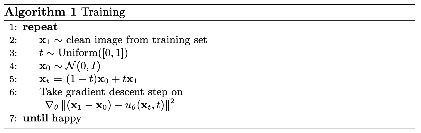
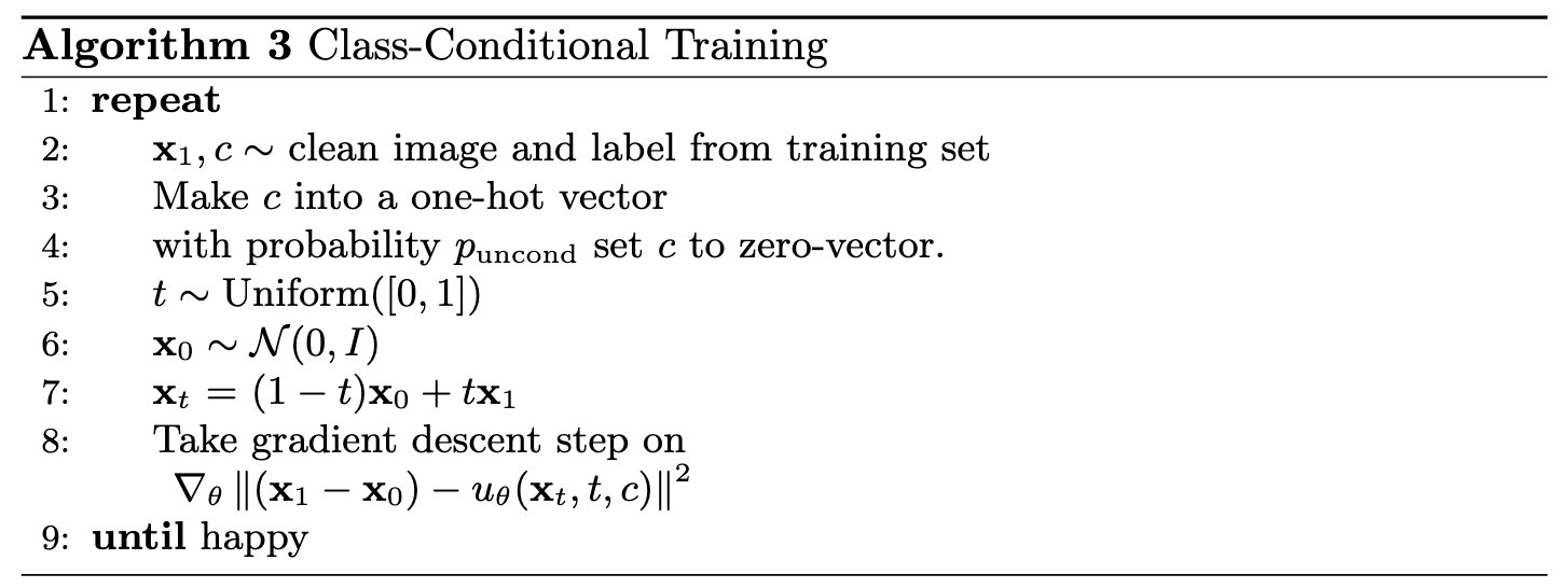
Training Algorithm
The training algorithm for the time-conditioned UNet is as follows:
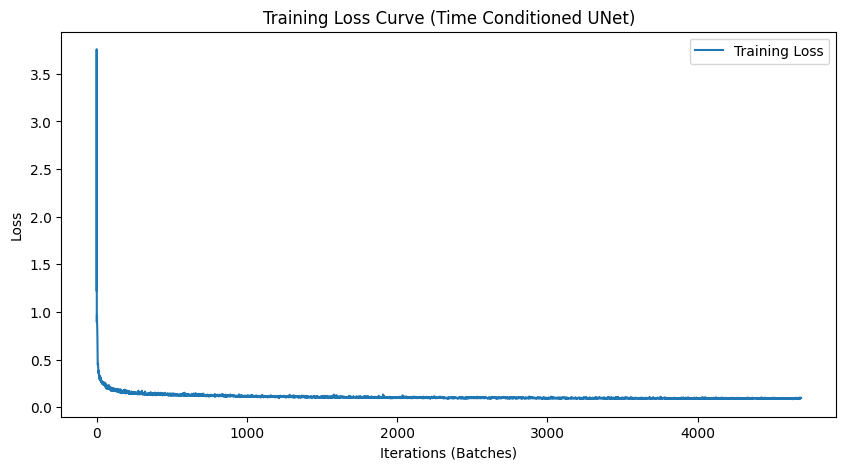
2.2 Training the UNet
We train the time-conditioned UNet on MNIST with batch size 64. The model uses hidden dimension D = 64, Adam optimizer with initial learning rate 1e-2, and an exponential learning rate decay scheduler with gamma = 0.95.
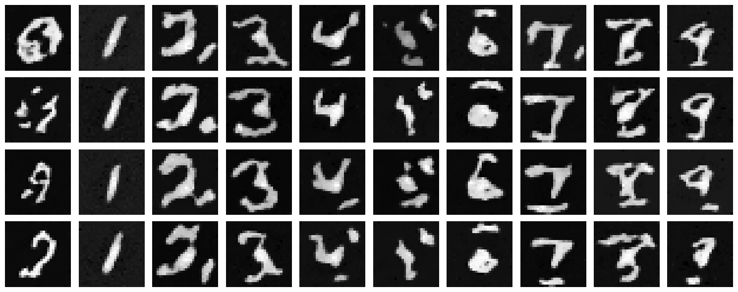
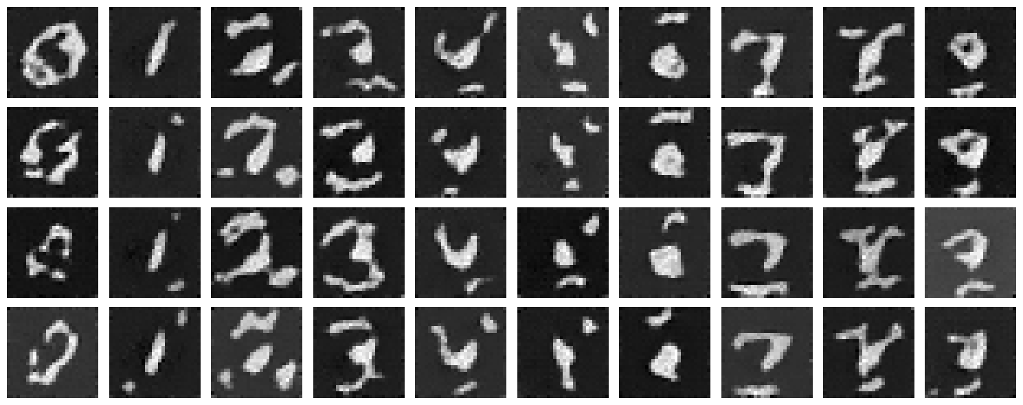
2.3 Sampling from the UNet
We can now use our UNet for iterative denoising. Starting from pure noise, we iteratively apply the learned flow to generate realistic digit images.
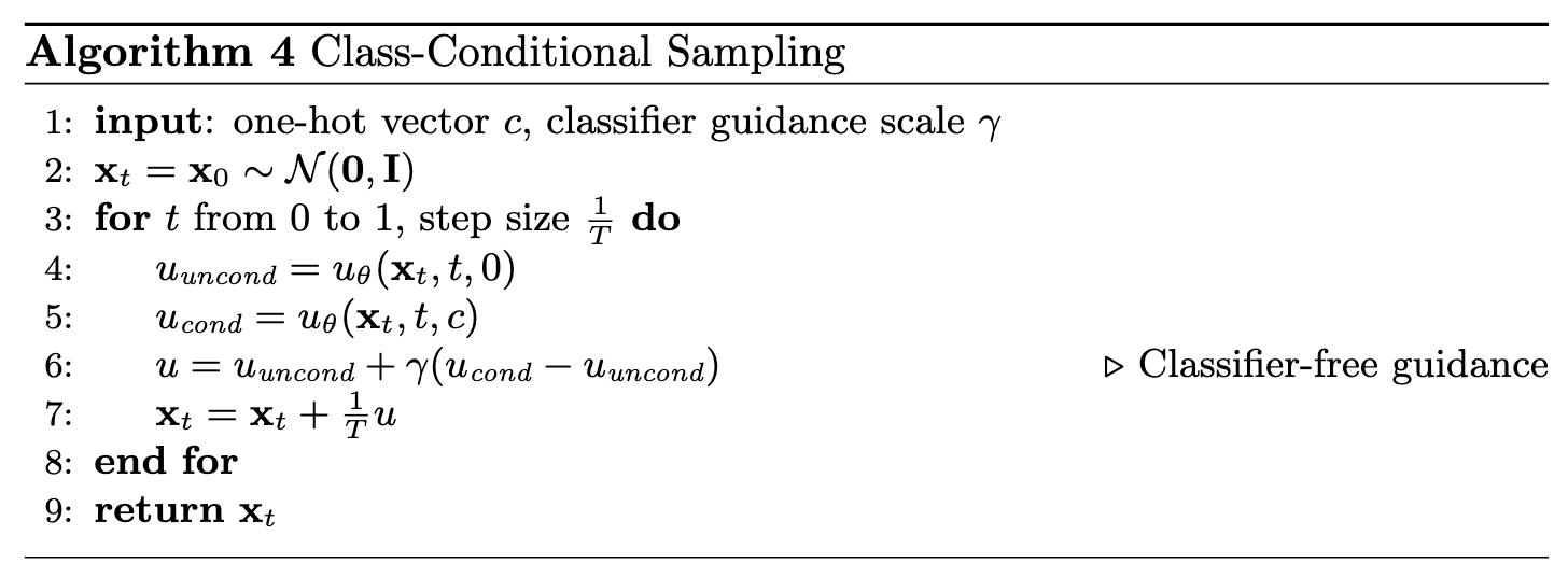
Sampling Algorithm
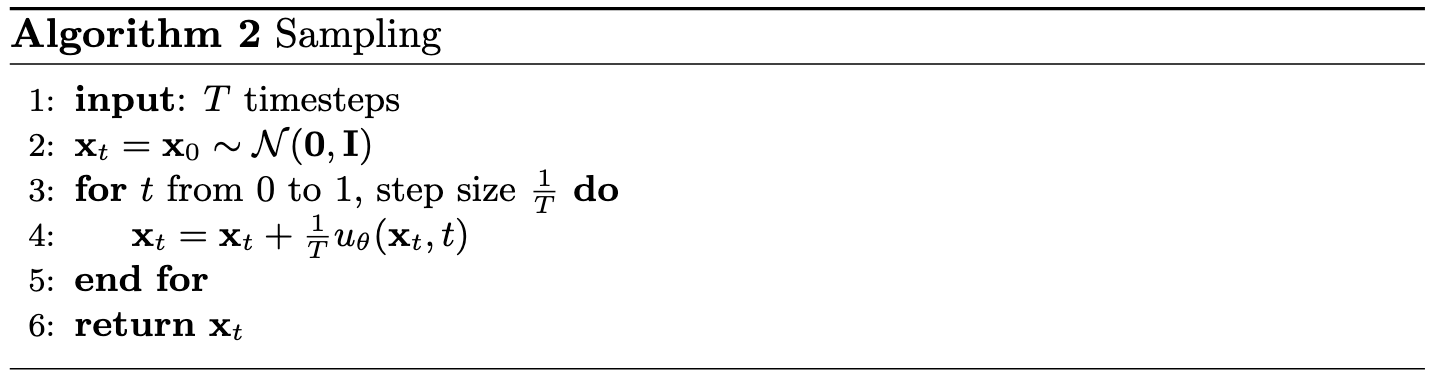
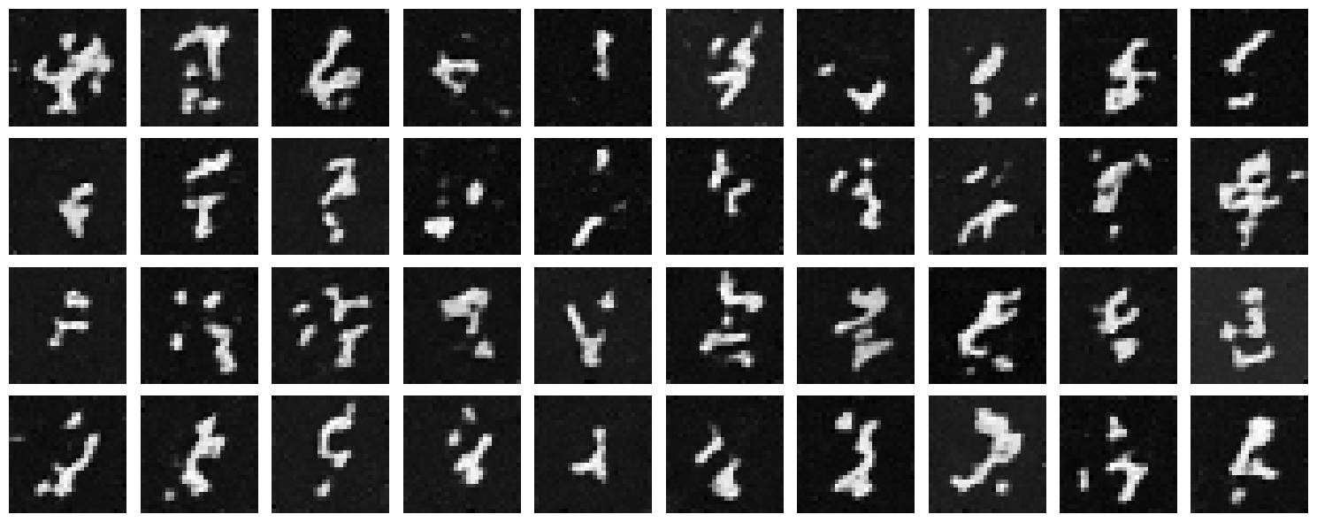
We can see our Unet reaches its performance plateau pretty quickly after 5 epochs. This is a good sign the Unet is learning the flow model reasonably well but there is still plenty of room for improvement. Since time conditioning helped our Unet, lets see if we can improve it further by adding class conditioning.
2.4 Adding Class-Conditioning to UNet
To improve results and give us more control for image generation, we condition our UNet on the class of the digit (0-9). We implement classifier-free guidance where 10% of the time we drop the class conditioning vector by setting it to 0.
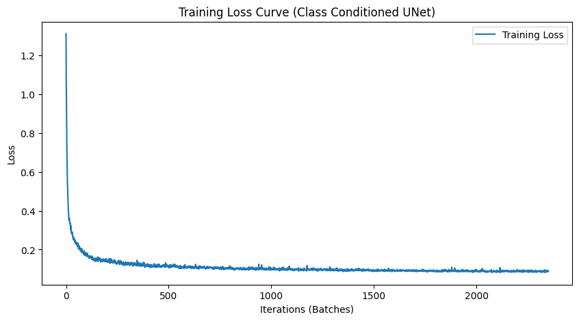
2.5 Training the UNet
Training for the class-conditioned UNet is similar to time-only conditioning, with the addition of class conditioning vectors and periodic unconditional generation. For this, we also introduced a dropout rate of 0.1 to the class conditioning vectors to help the Unet learn the flow model better and prevent overfitting.
Training Algorithm
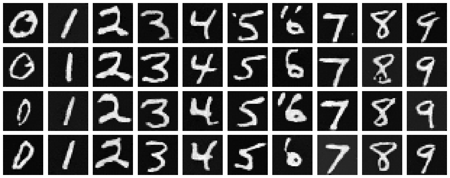
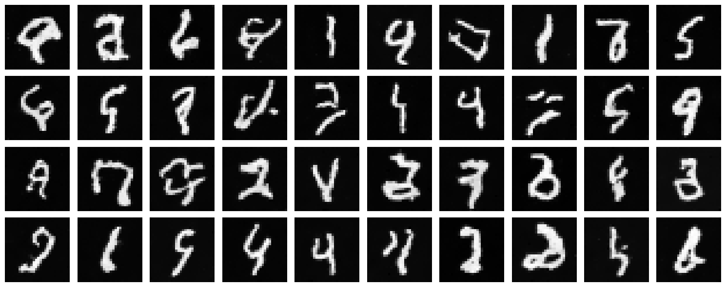
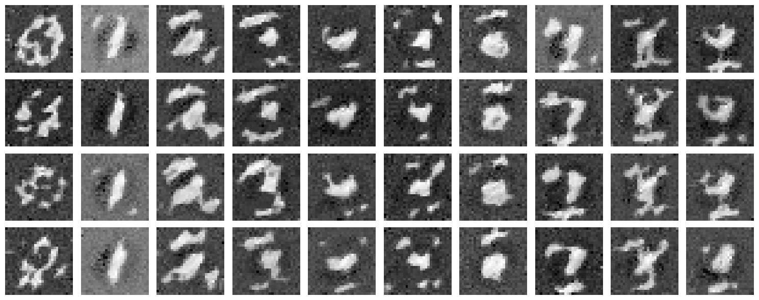
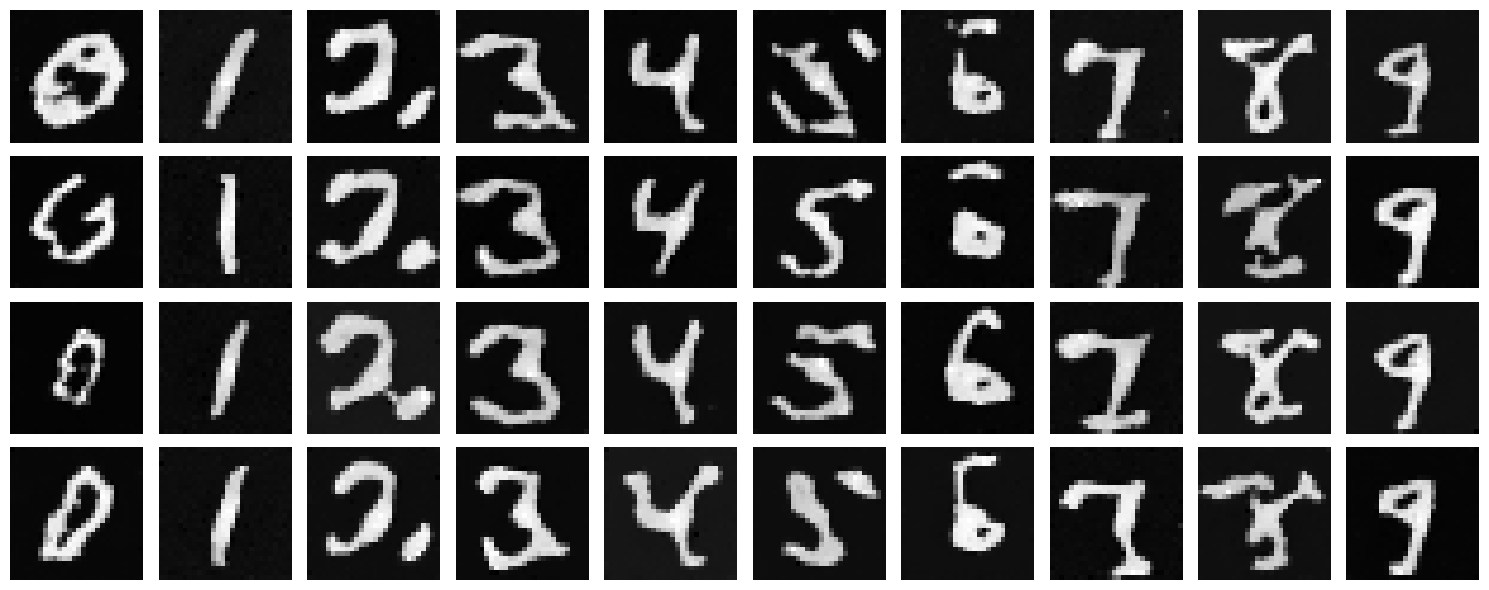
2.6 Sampling from the UNet
We sample with class-conditioning and use classifier-free guidance with guidance scale $\gamma = 1.5$.
Sampling Algorithm
With Learning Rate Scheduler
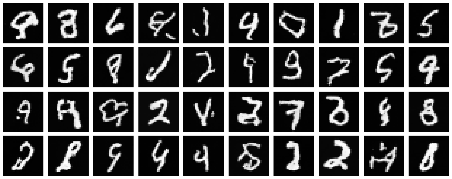
Without Learning Rate Scheduler (AdamW Optimizer)
We removed the exponential learning rate scheduler and compensated by using the AdamW optimizer, which provides better weight decay and can help maintain performance without explicit learning rate decay.
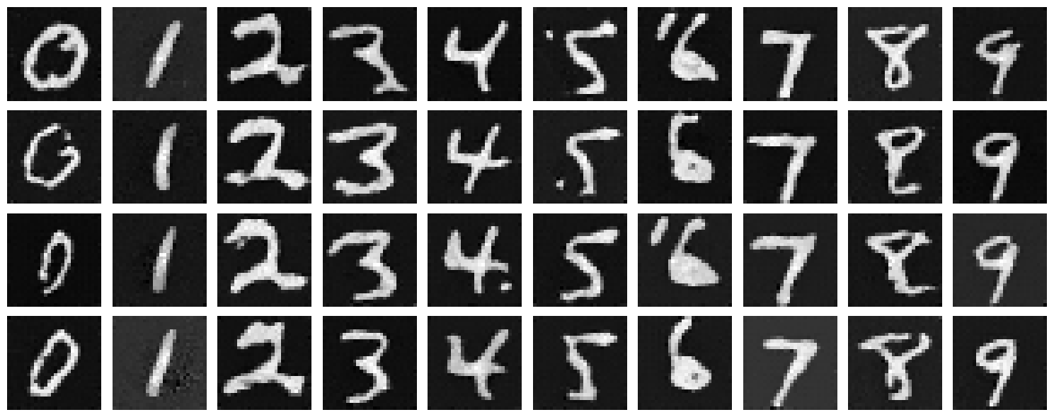
Compensation Strategy
To maintain performance without the learning rate scheduler, we switched from Adam to AdamW optimizer. AdamW provides better weight decay handling and can achieve similar convergence behavior through its adaptive learning rate mechanism. The results show that we can achieve comparable quality without explicit learning rate decay, simplifying the training setup while maintaining performance.
We can see the class-conditioned UNet performs significantly better than the time-conditioned UNet. This is a good sign that class conditioning is helping the Unet learn the flow model better. Lets see if we can improve it further by adding more conditioning. We can also see that the learning rate scheduler was hindering performance, and switching to Adam with weight decay helped achieve better results.
We have successfully trained a flow matching model that can denoise images and generate realistic digit images!