Project Overview
This project explores fundamental concepts in digital image processing, focusing on spatial domain filtering, frequency domain analysis, and image blending techniques. The project is divided into two main parts: Part 1 focuses on building intuitions about 2D convolutions and filtering, while Part 2 explores frequency domain processing, hybrid images, and multiresolution blending.
Part 1: Fun with Filters
In this part, we build intuitions about 2D convolutions and filtering, beginning with the humble finite difference filters in the x and y directions. These allow us to detect vertical and horizontal edges respectively.
Part 1.1: Convolutions from Scratch!
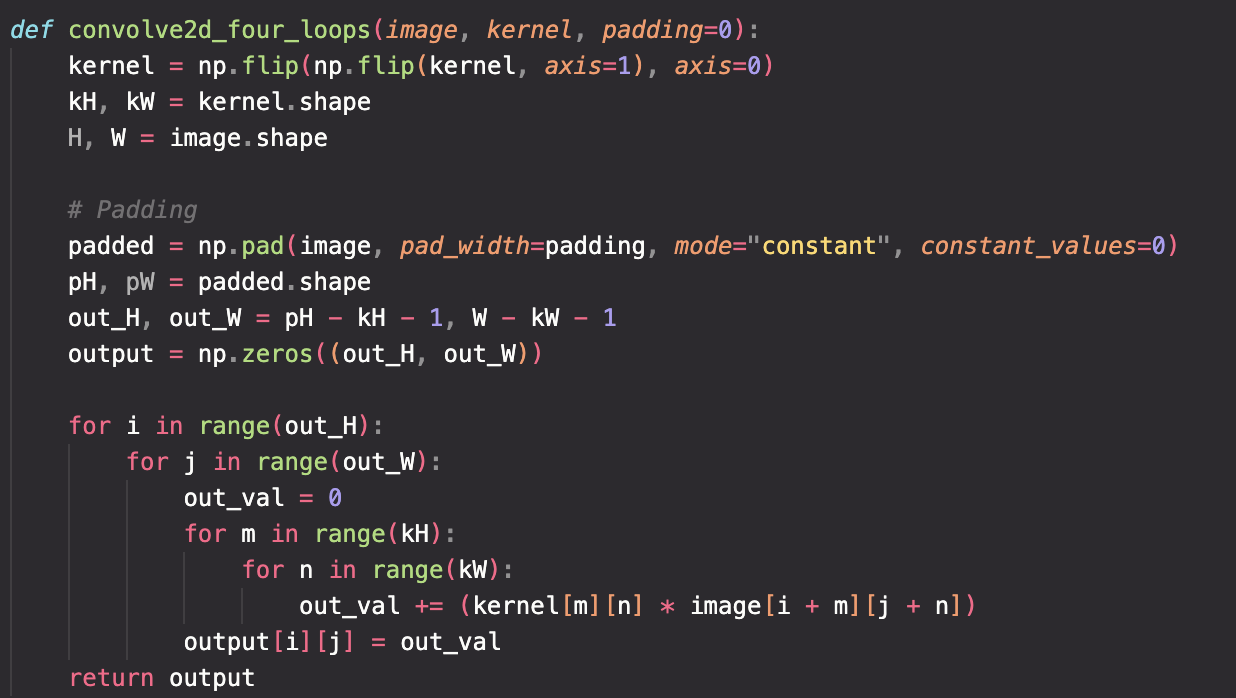
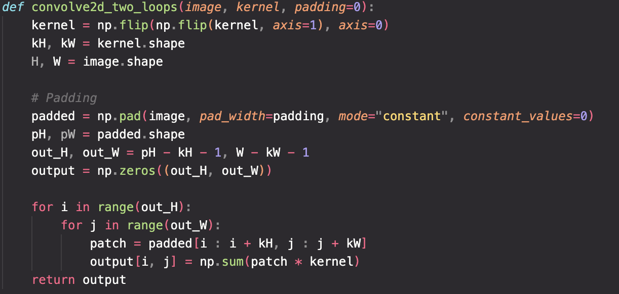
First as a recap to convolution, I implemented an implementation with two four loops and four for loops to compare and contrast the runtime performance of the convolution operations. I also compared these implementations with the built-in convolution function scipy.signal.convolve2d.
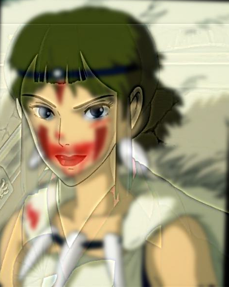
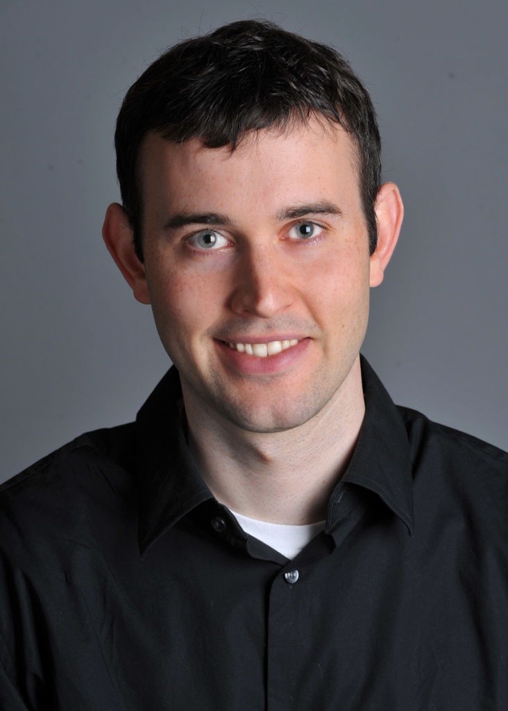
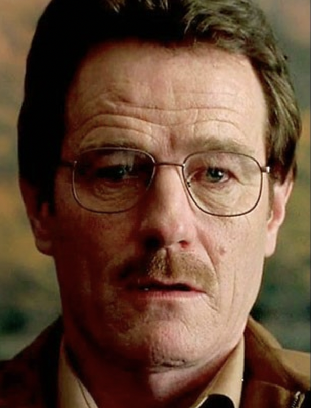
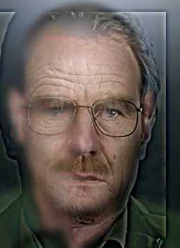
I took a picture of myself (read as grayscale), wrote out a 9x9 box filter, and convolved the picture with the box filter. I also applied the finite difference operators Dx and Dy.
Code Implementation Comparison
Runtime Performance Comparison
After averaging the results across 5 experiments, we can see that scipy is significantly faster due to numerical optimizations and proper vectorization. It is also worth noting that the extra cost of having to compute a patch by patch dot product slows down the four loop implementation significantly.
| Implementation | Average Time |
|---|---|
| Two Loops | 55.9 seconds |
| Four Loops | 581.1 seconds |
| Scipy | 2.1 seconds |
Image Processing Results
To begin apply convolutions to images, I first applied a 9x9 box filter, a finite difference operator D_x, and a finite difference operator D_y to my self portrait. The finite difference operators are defined as:
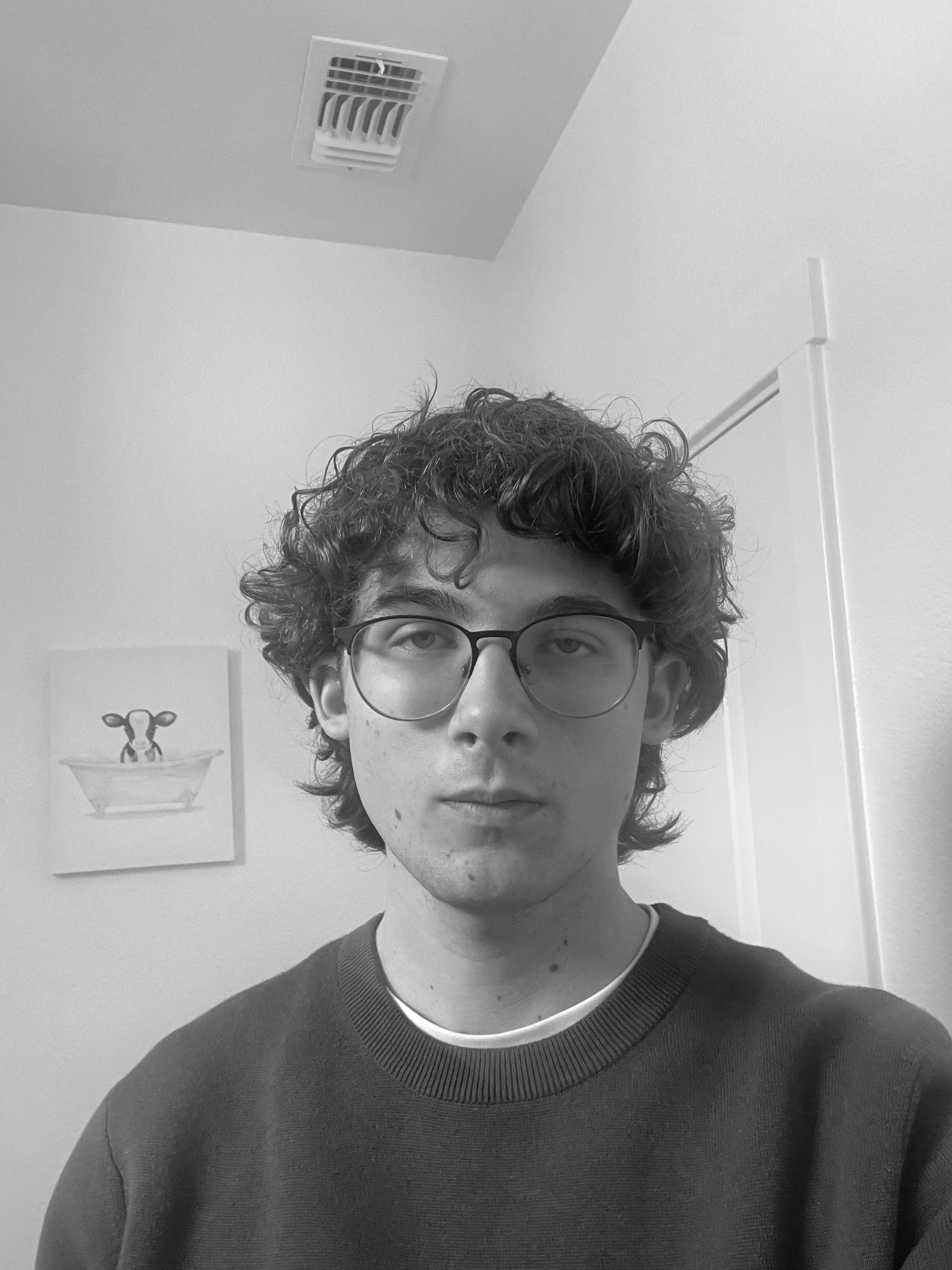
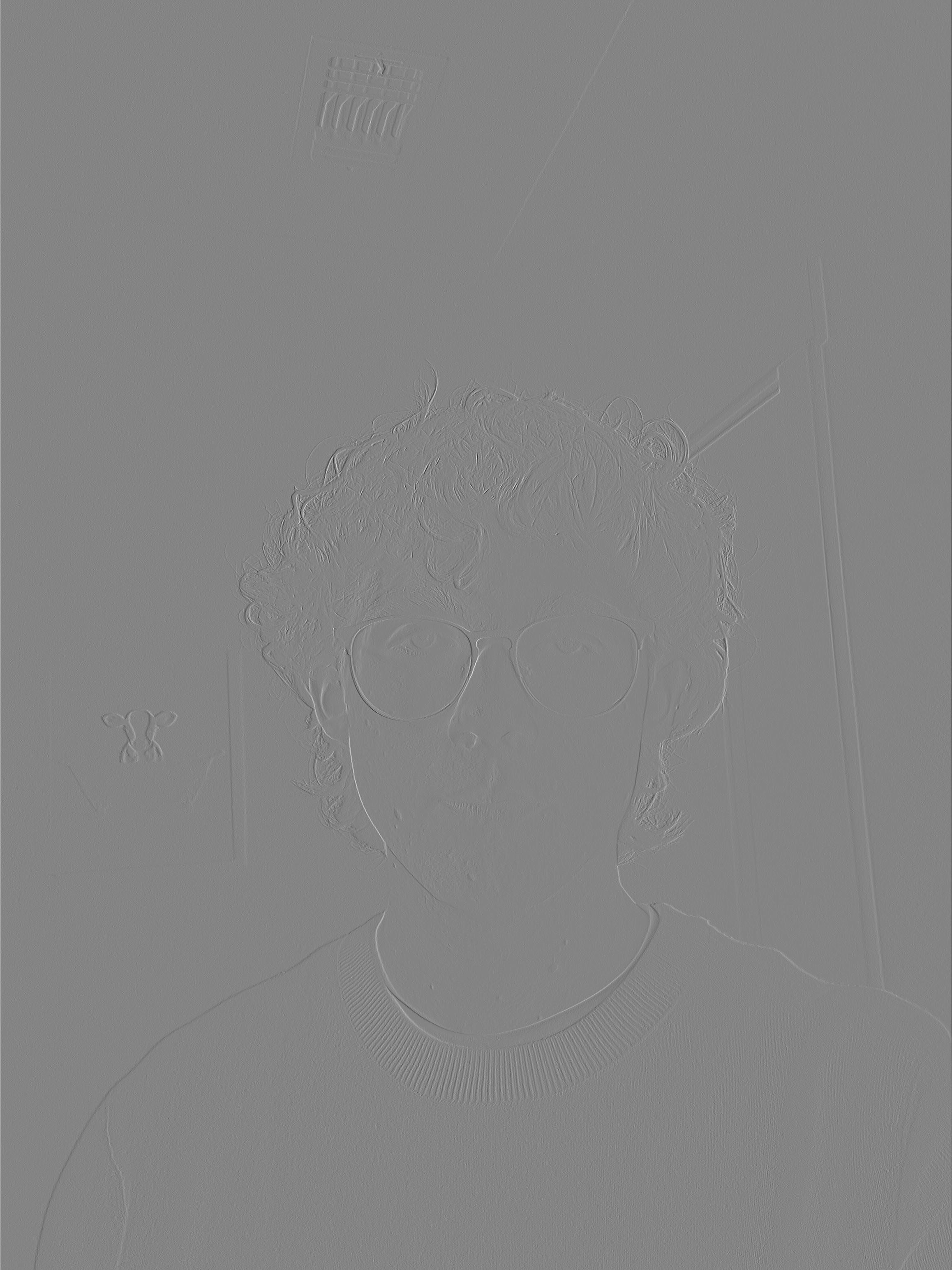

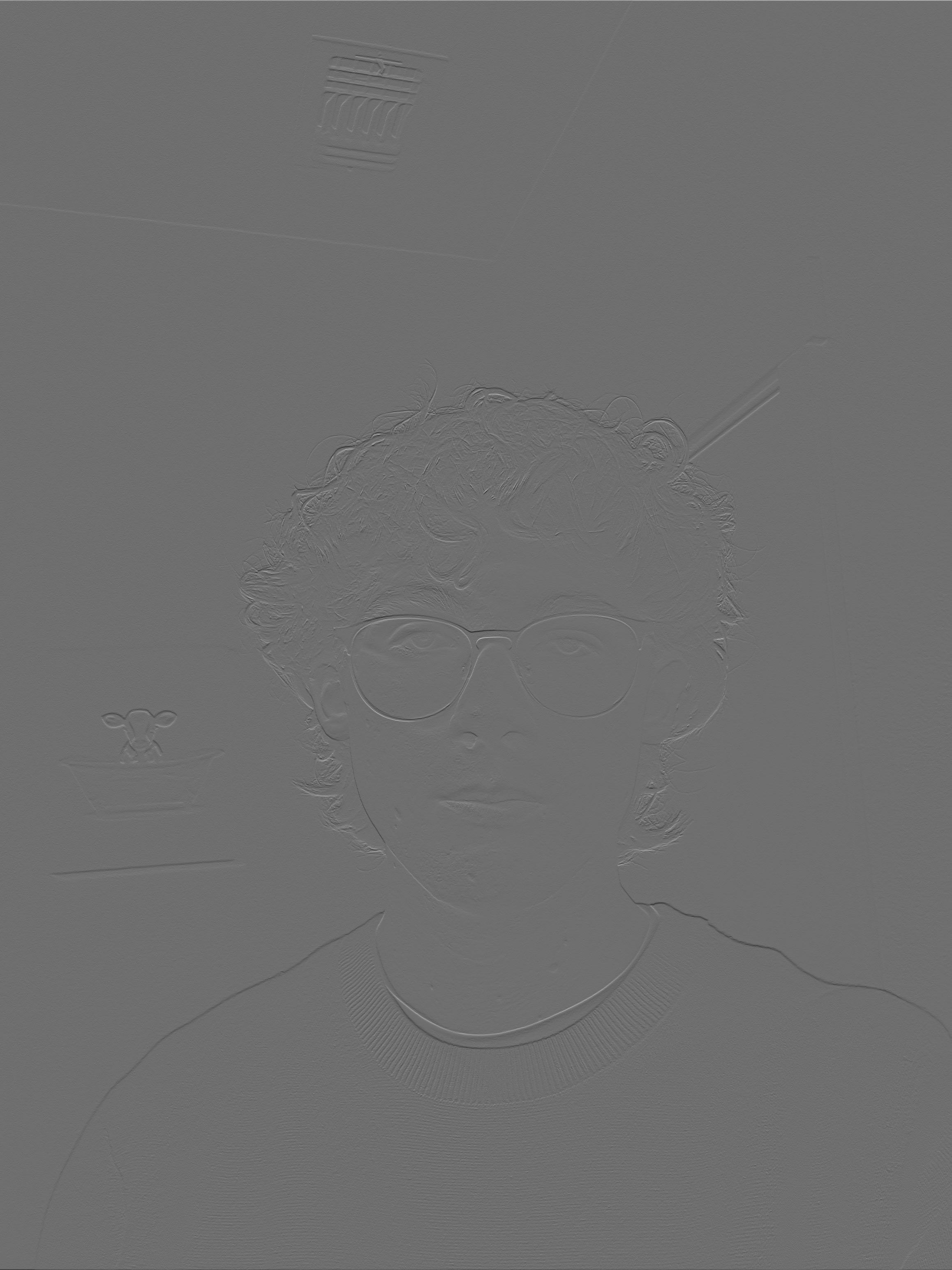
We can see the box filter as a simple, but effective low pass filter resulting in a blurred image due to averaging out the pixel values. We can also see the finite difference operators as simple edge detectors for horizontal and vertical edges. For proper edge detection however, we need to use a more sophisticated operator.
Part 1.2: Finite Difference Operator
Lets move on to proper edge detection. We can convolve this image of "The Cameraman" with the finite difference operators D_x and D_y. This gives us once again simple horizontal and vertical edge detection. Next, we can combine the results of each of these operators through the gradient magnitude defined below where Ix and Iy are the images resulting from the finite difference operators:
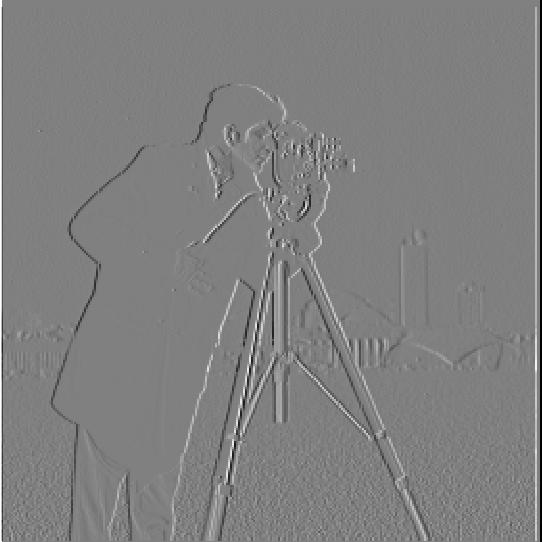
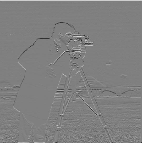
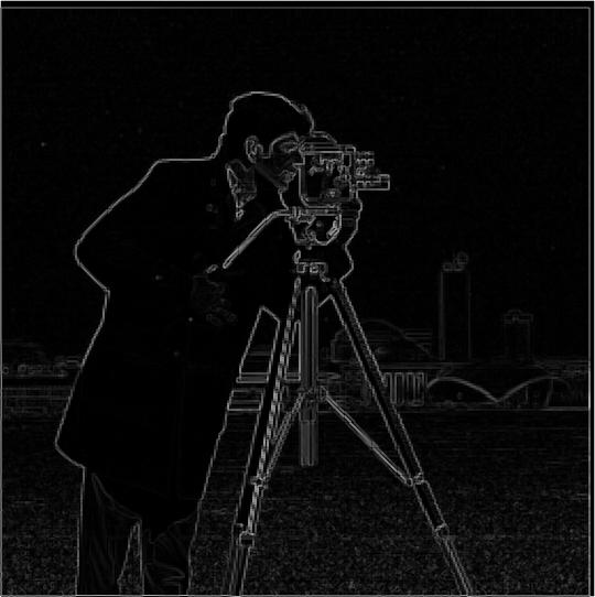
Threshold Selection: I chose a threshold that balances finding all real edges while suppressing noise. For the above images, thresholding at 3e-1 was a good balance between finding all edges and suppressing noise.
Part 1.3: Derivative of Gaussian (DoG) Filter
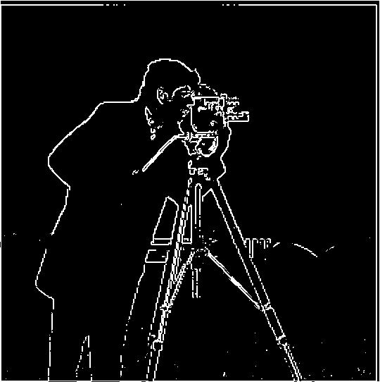
Even with threshold tuning, the results with just the gradient magnitude were rather noisy. Luckily, a gaussian filter can be used to smooth the image before applying the graident magnitude. Not only this but through the properties of convolution, this is equivelant to convolving with the derivative of the gaussian filter which means we only need to convolve a filter with an image once in each respective direction!
We can see the results of applying these filters is a much smoother and sharper edge detection then before. Additionally the two methods result in the exact same image. We have made a pretty nice edge detector simply through convolution!

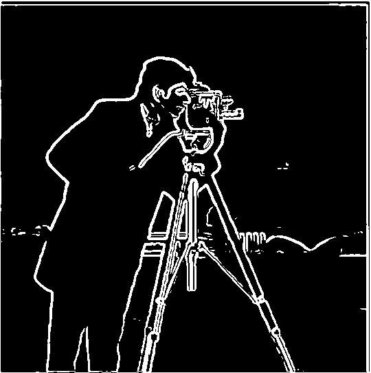
cv2.getGaussianKernel() to create 1D Gaussian kernels and took the outer product to create 2D Gaussian filters. The DoG filters were created by convolving the Gaussian with D_x and D_y operators.
DoG Filter Components


Part 2: Fun with Frequencies!
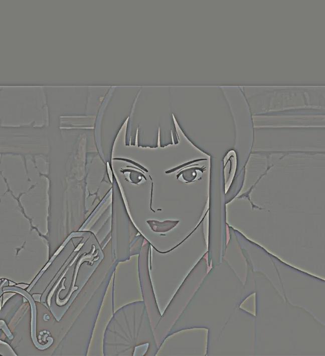
Part 2.1: Image "Sharpening"
We can also use convolution and gaussian filters to sharpen images. Because the gaussian filter is a low pass filter that retains only low frequencies, by subtracting the blurred version of an image from an original image we get the high frequencies. Adding these with a scalar factor, alpha, to the original image allows us to artificially introduce high frequency features resulting in images looking sharper.
This combines into a single convolution operation called the unsharp mask filter.
Sharpening Results with Different Alpha Values
Original Images and High Frequency Components

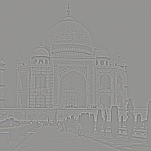

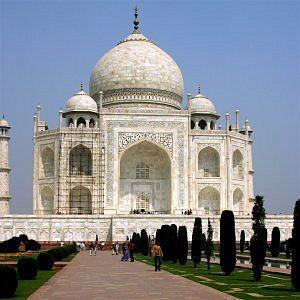
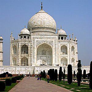
Taj Mahal Sharpening Results


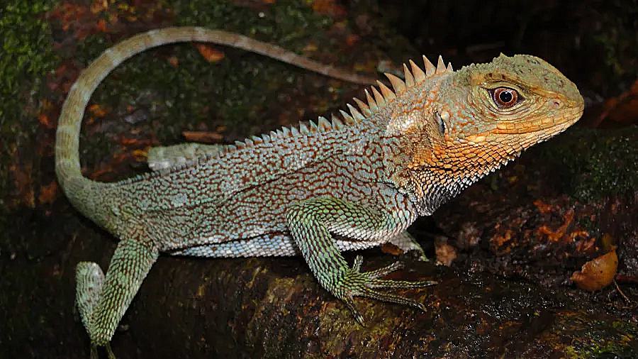
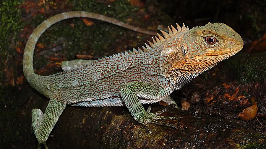
Lizard Sharpening Results


Note: It should be noted this technique is cheating a bit. By adding in scaled high frequency features to the image, we are not actually adding any new information that "sharpens" the image. Noneoftherefore, the effect is still noticeable and a useful enhancemnet that is very common in cheaper cameras.
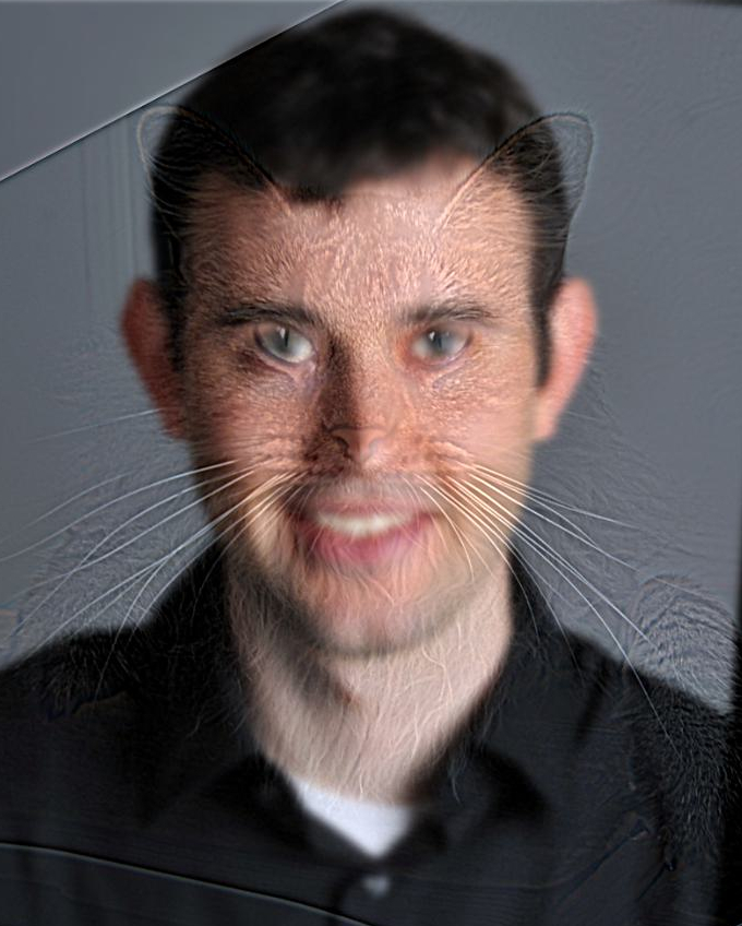
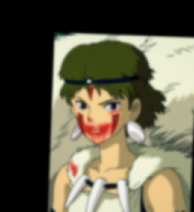
Part 2.2: Hybrid Images
Hybrid images are static images that change in interpretation as a function of viewing distance. Because high frequencies tend to dominate human perception whenver available, but low frequency (smoother) parts of images appear at a distance, it is possible to construct images that are composed of two images. One seen further away, and the other seen only up close. This technique is based off the SIGGRAPH 2006 paper by Oliva, Torralba, and Schyns and can be used to create some extremely interesting results.
Hybrid Image Results

Frequency Analysis
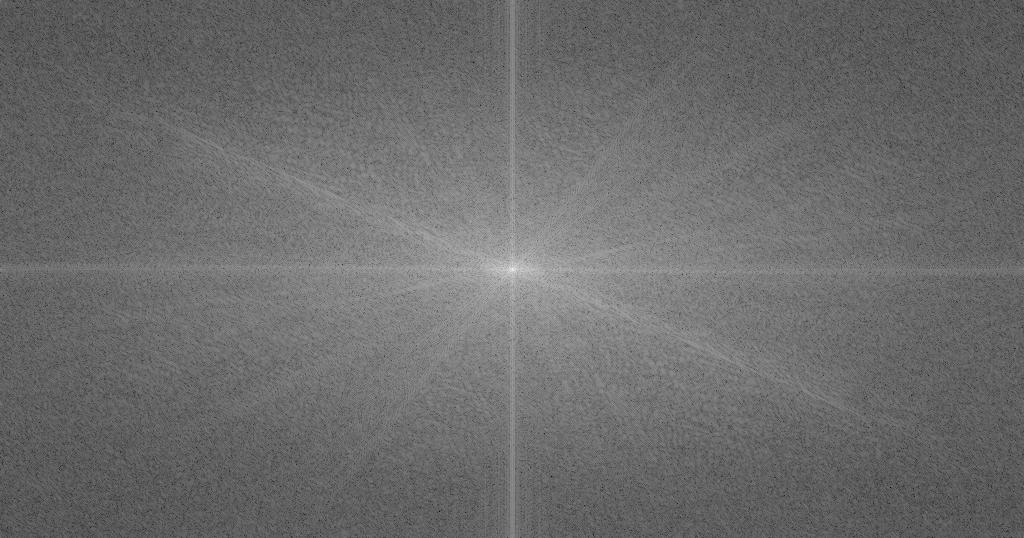
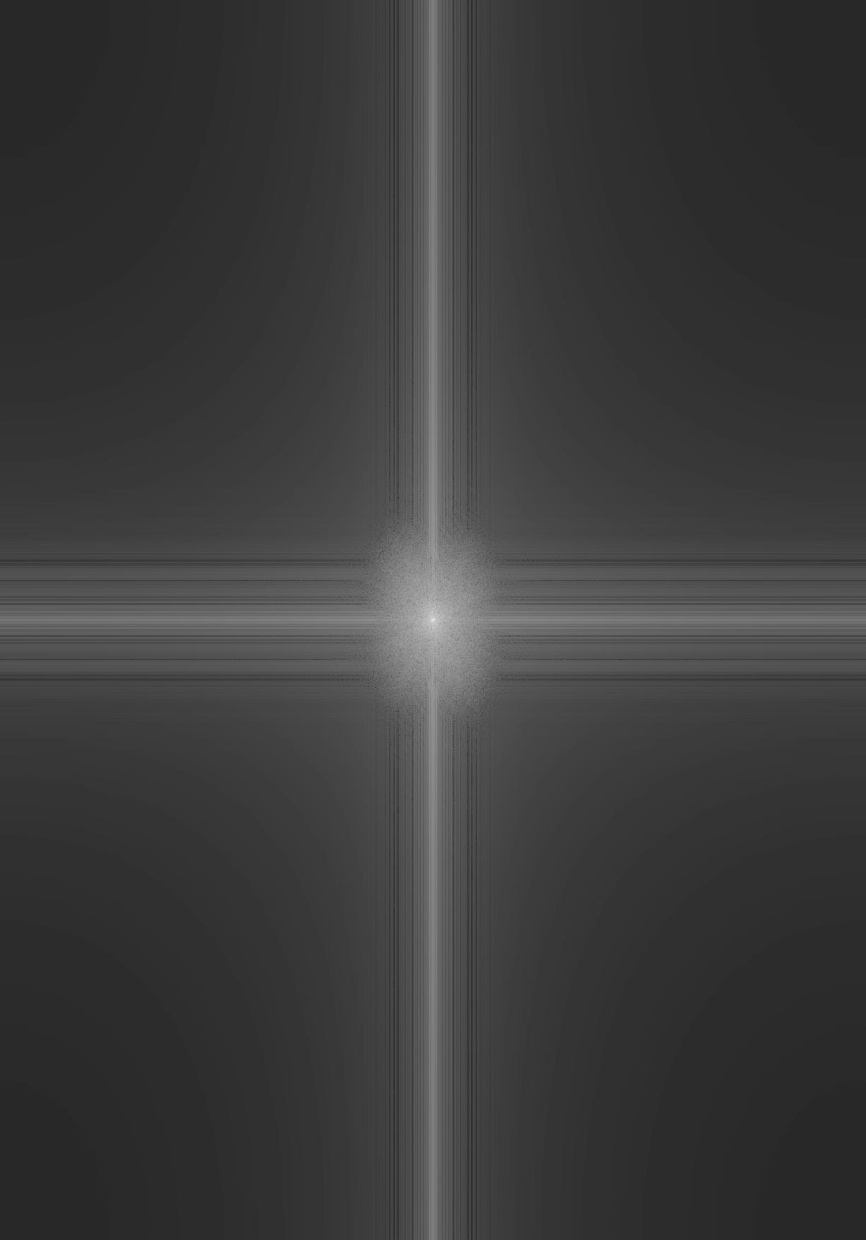
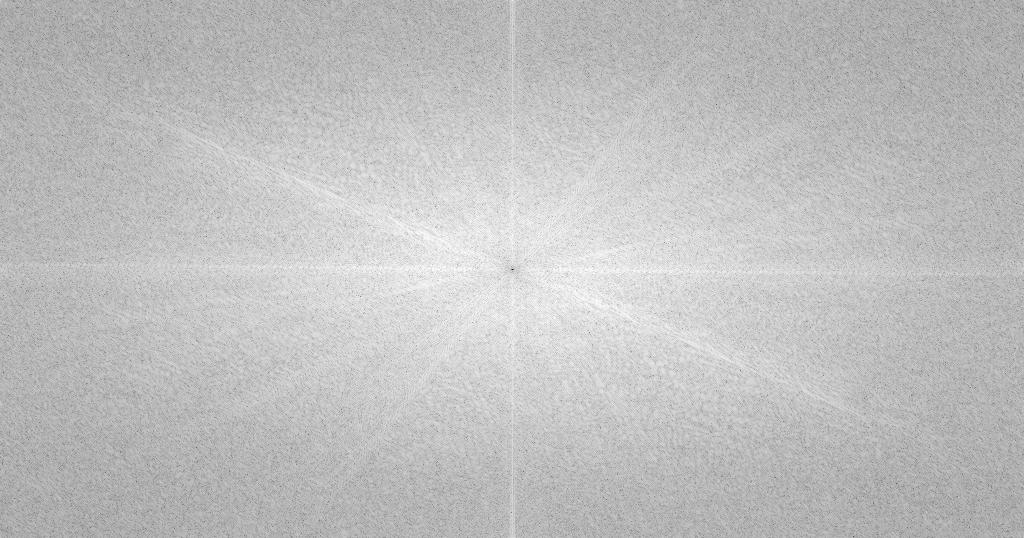
For my favorite result (San + Eboshi), I illustrate the process through frequency analysis:
Original Images and Their Frequency Components
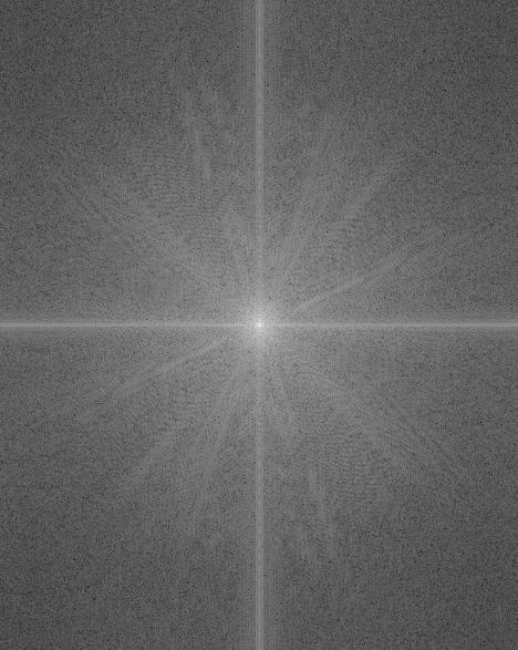
Post-Filtered Images and Their Frequency Spectra
Cutoff Frequency Choice
For the San/Eboshi hybrid, I carefully selected the cutoff frequencies to achieve optimal blending:
- Low Pass Filter (San): σ = 4.0 - This preserves the smooth, low-frequency features of San's face while removing fine details
- High Pass Filter (Eboshi): σ = 3.5 - This retains the sharp, high-frequency details of Eboshi's features while removing the smooth background
The choice of these sigma values was determined through experimentation to find the optimal balance between preserving important facial features and achieving seamless blending in the final hybrid image.
Implementation Note: In order to create hybrid images, it was necessary to "align" images so San's eyes can overlay Eboshi's eyes. This results in a slight rotation as seen by the post low pass filtered image. This also means I cropped the final image so it appears more clean.
Final Hybrid Result
Part 2.3: Gaussian and Laplacian Stacks
An exciting application of Gaussian filters and frequency analysis is that it can be combined to create seamless image blending. A gaussian stack can be built by applying a gaussian filter at different scales to the same image. A laplacian stack can then be created by subtracting each level of the gaussian stack from the next lower level. Since Gaussian filters are low pass filters, this resulting difference gives an image composed of frequencies in a particular band allowing us to progressivley blend two images together. The resulting stack from the differences is known as a Laplacian stack. Each level L_i of the stack can be described by the following:
This process of image blending is described in detail in Burt & Adelson (1983).
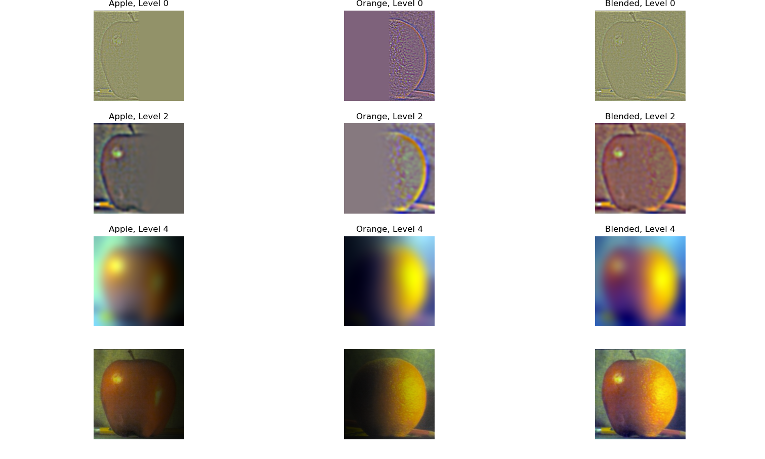
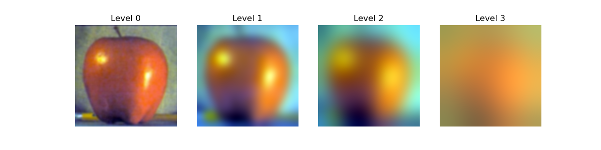
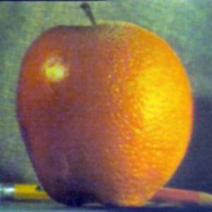
To start, I recreated Figure 3.42 in Szelski's book to show the process of image blending using Gaussian and Laplacian stacks on the famous "Oraple" example. We can see that as we go down the stack the image becomes inceasingly blurred due to reaching lower and lower frequency bands. This is seen in the first 3 rows of the below figure. The final row are the weighted image blends of each image and the final result.
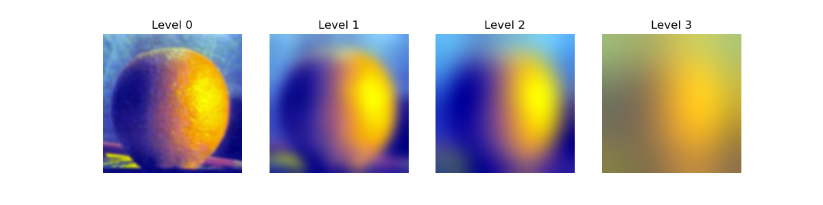
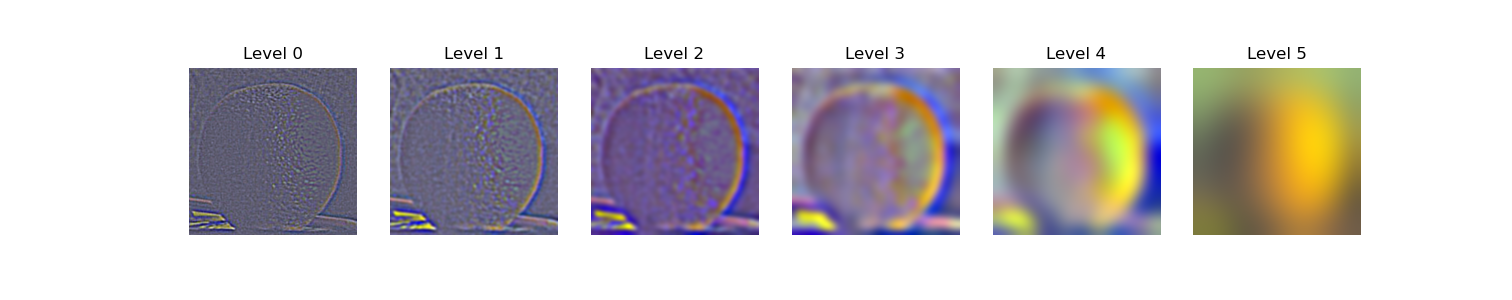
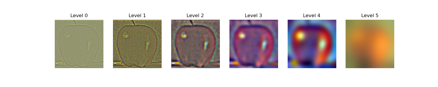
We can also visualize the Gaussian and Laplacian stacks directly for a stack with more levels. It is important to note the very last level of the stack is the image with the lowest frequencies. Additionally, I used a larger laplacian stack here to show the results more clearly.
Gaussian and Laplacian Stacks
Gaussian Stacks
Laplacian Stacks
Part 2.4: Multiresolution Blending (a.k.a. the Oraple!)
Finally, I implemented multiresolution blending described in the paper using these laplacian stacks. For each blend, I take a mask and alpha blend two images together with an increasingly blurrier mask as we go down the stack. This results in a seamless blend of two images. Mathematically, this can be described below for each level of the blended stack we reconstruct.
Mathematical Foundation of Alpha Blending
For each level i of the blend stack, the blended Laplacian level is calculated as:
where:
- $L_i^{(1)}$ and $L_i^{(2)}$ are the i-th levels of the Laplacian stacks for images 1 and 2
- $M_i$ is the i-th level of the Gaussian mask stack (increasingly blurred)
- $(1 - M_i)$ represents the complementary mask
The final blended image is reconstructed by summing all blended levels: $I_{final} = \sum_{i=0}^{n} L_i^{blend}$, then normalized to [0,1] range.
Oraple - The Classic Blend
Custom Blended Images
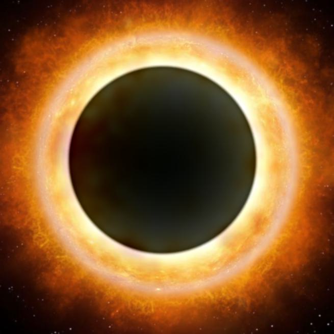
Additionally, I created a few custom blended images using irregular masks to demonstrate the power of multiresolution blending:
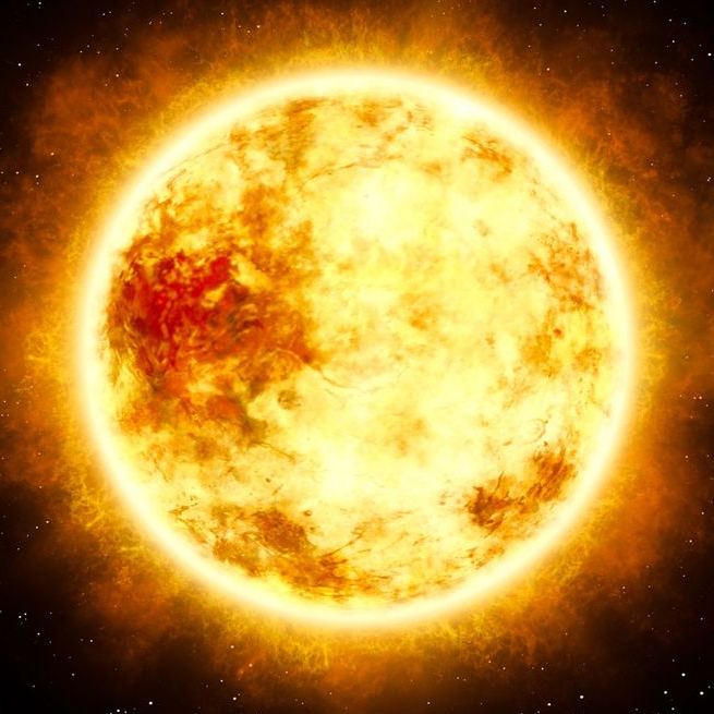
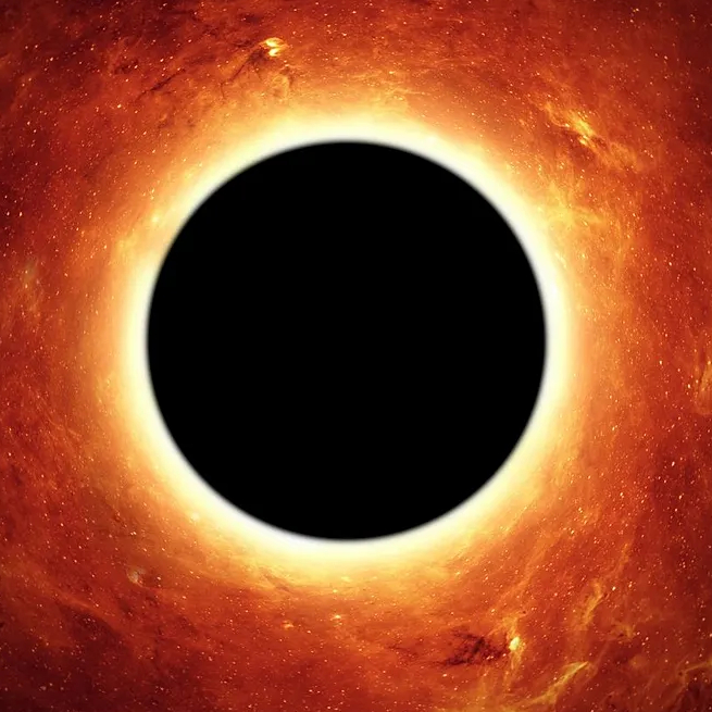
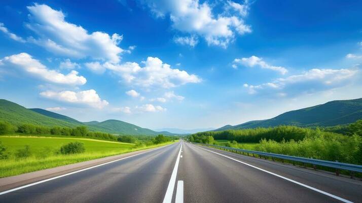
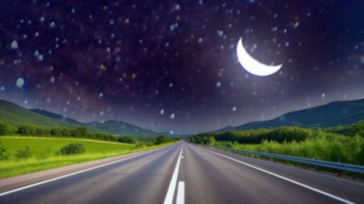
Black Hole Sun

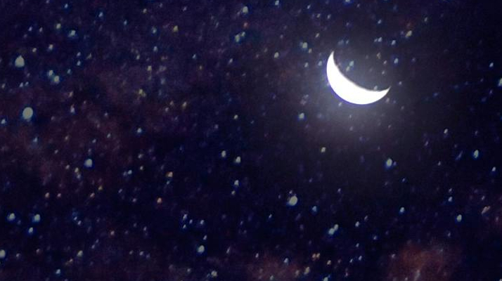
Night Sky Road

Conclusion
This project provided comprehensive hands-on experience with fundamental image processing techniques, from basic spatial filtering to advanced frequency domain operations and multiresolution blending. The combination of theoretical understanding and practical implementation revealed the elegance and power of digital image processing algorithms.
The project successfully demonstrated how different filtering approaches can be used for various applications, from edge detection to image enhancement and creative compositing. The multiresolution blending technique proved particularly effective for creating seamless image composites, while hybrid images showcased the fascinating intersection of computer vision and human perception.