Neural Radiance Fields (NeRF)

Project Overview

This project explores Neural Radiance Fields (NeRF), a state-of-the-art technique for novel view synthesis that represents 3D scenes as continuous volumetric functions. The project is divided into multiple parts, starting with camera calibration and 3D object scanning, moving into fitting a neural field to a 2D image, and finally fitting a neural radiance field from multi-view images.

This technology and implementation is based on NeRF from UC Berkeley.

Part 0: Calibrating Your Camera and Capturing a 3D Scan

For the first part of the assignment, we take a 3D scan of an object which will be used to build a NeRF model later. This process uses visual tracking targets called ArUco tags, which provide a reliable way to detect the same 3D keypoints across different images. There are 2 main components: 1) calibrating camera parameters, and 2) using them to estimate camera pose.

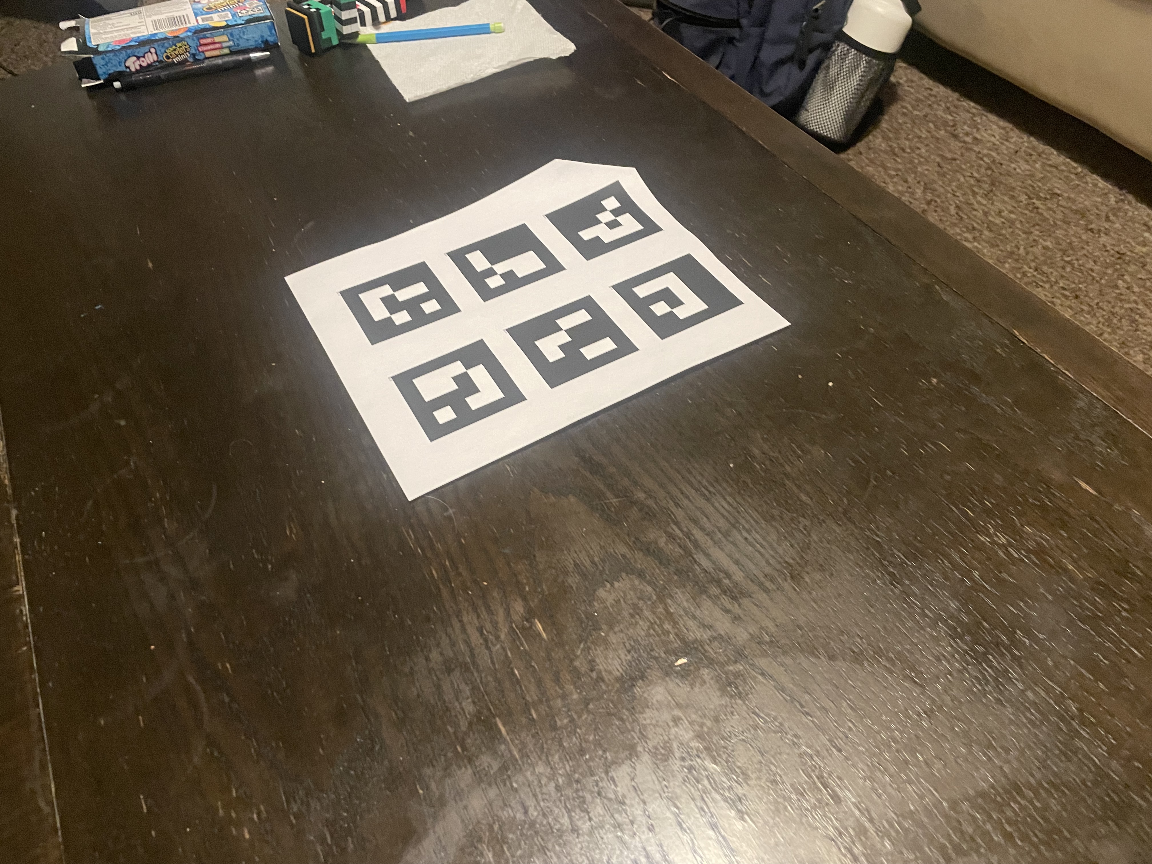
Part 0.1: Calibrating Your Camera

The first step in the pipeline is camera calibration, which involves capturing 30-50 images of calibration tags (ArUco markers) from different angles and distances, similar to traditional chessboard calibration. The calibration process loops through all calibration images, detects ArUco tags using OpenCV's ArUco detector with cv2.aruco.getPredefinedDictionary() and cv2.aruco.DetectorParameters(), extracts corner coordinates from detected tags, and collects all detected corners along with their corresponding 3D world coordinates. Finally, cv2.calibrateCamera() is used to compute the camera intrinsics matrix and distortion coefficients from the collected 2D-3D correspondences.

The ArUco tag detection process follows these steps:

• Create an ArUco dictionary using cv2.aruco.getPredefinedDictionary(cv2.aruco.DICT_4X4_50) for 4x4 tags
• Initialize detector parameters with cv2.aruco.DetectorParameters()
• Detect markers in each image using cv2.aruco.detectMarkers(), which returns:
  • corners: list of length N (number of detected tags), each element is a numpy array of shape (1, 4, 2) containing the 4 corner coordinates
  • ids: numpy array of shape (N, 1) containing the tag IDs for each detected marker
• Process detected corners only when ids is not None, skipping images with no detections

Example calibration image showing ArUco tags used for camera calibration

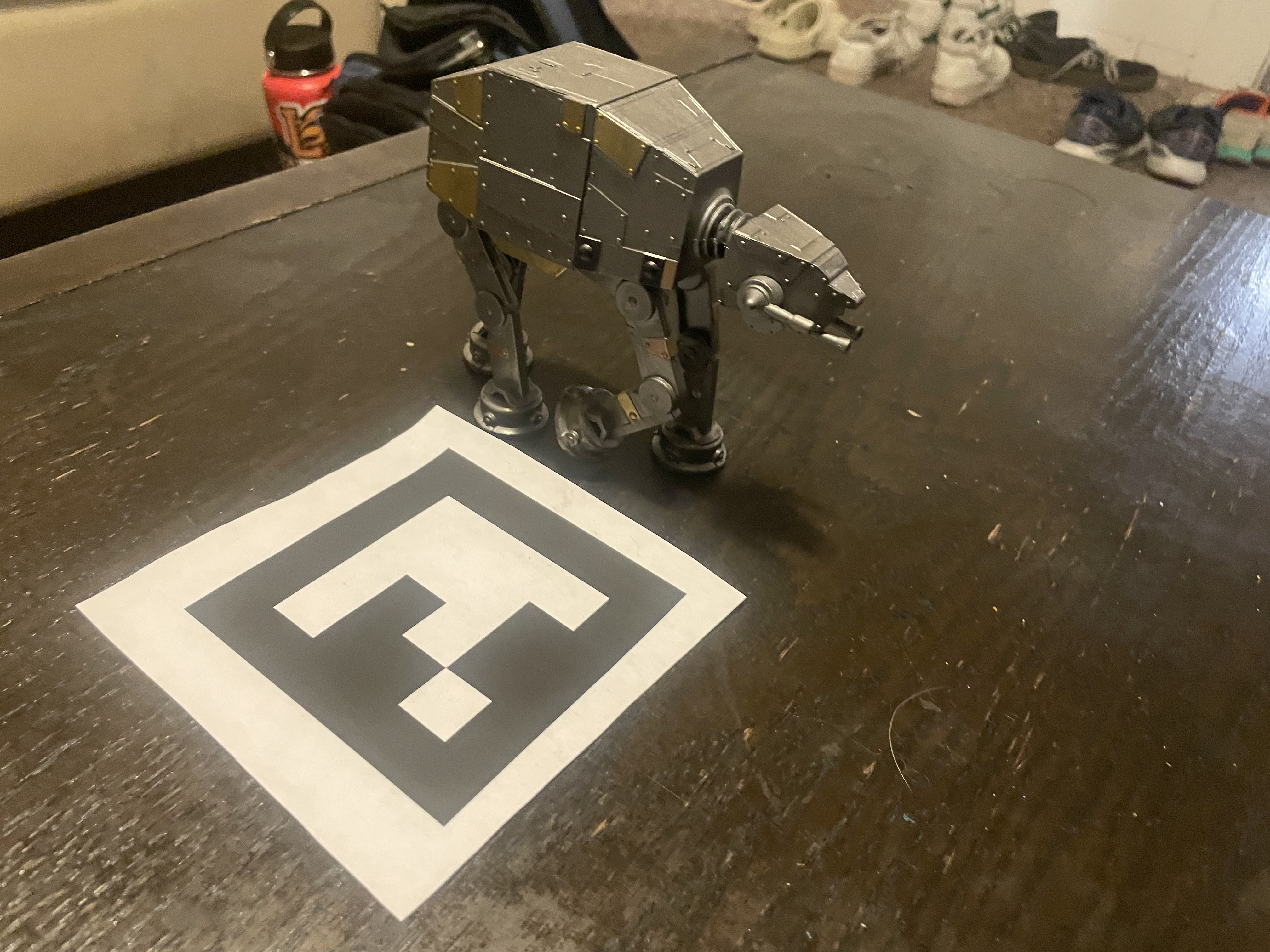
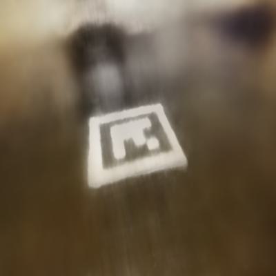
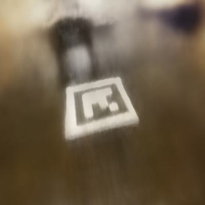
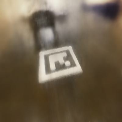
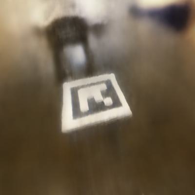
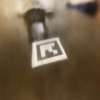
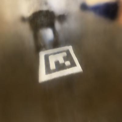
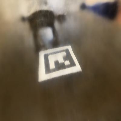
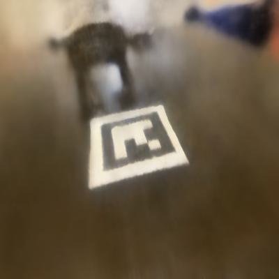
Part 0.2: Capturing a 3D Object Scan

After calibration, we capture a 3D scan by placing a single printed ArUco tag next to the object and taking 30-50 images from various angles using the same camera settings. To ensure good NeRF quality, images are captured at a uniform distance (10-20cm) with the object filling ~50% of the frame, avoiding exposure changes and motion blur.

Example object scan image showing the ATAT walker with ArUco tag for pose estimation

Part 0.3: Estimating Camera Pose

Once the camera is calibrated, we can use the intrinsic parameters to estimate the camera pose (position and orientation) for each image of the object. This is the classic Perspective-n-Point (PnP) problem: given a set of 3D points in world coordinates and their corresponding 2D projections in an image, we want to find the camera's extrinsic parameters (rotation and translation).

For each image in the object scan, the process involves:

• Detecting the single ArUco tag in the image
• Using cv2.solvePnP() to estimate the camera pose
• Converting the rotation vector to a rotation matrix using cv2.Rodrigues()
• Inverting the world-to-camera transformation to get the camera-to-world (c2w) matrix

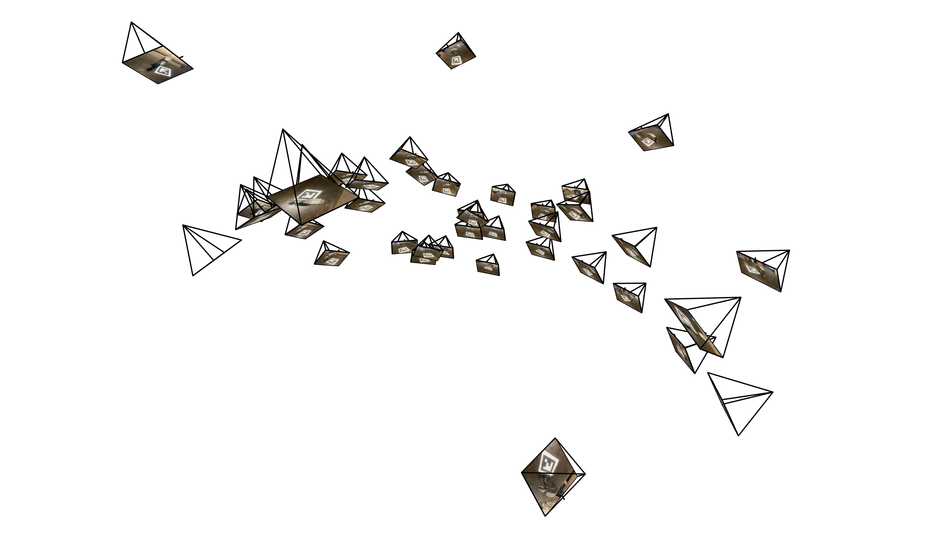
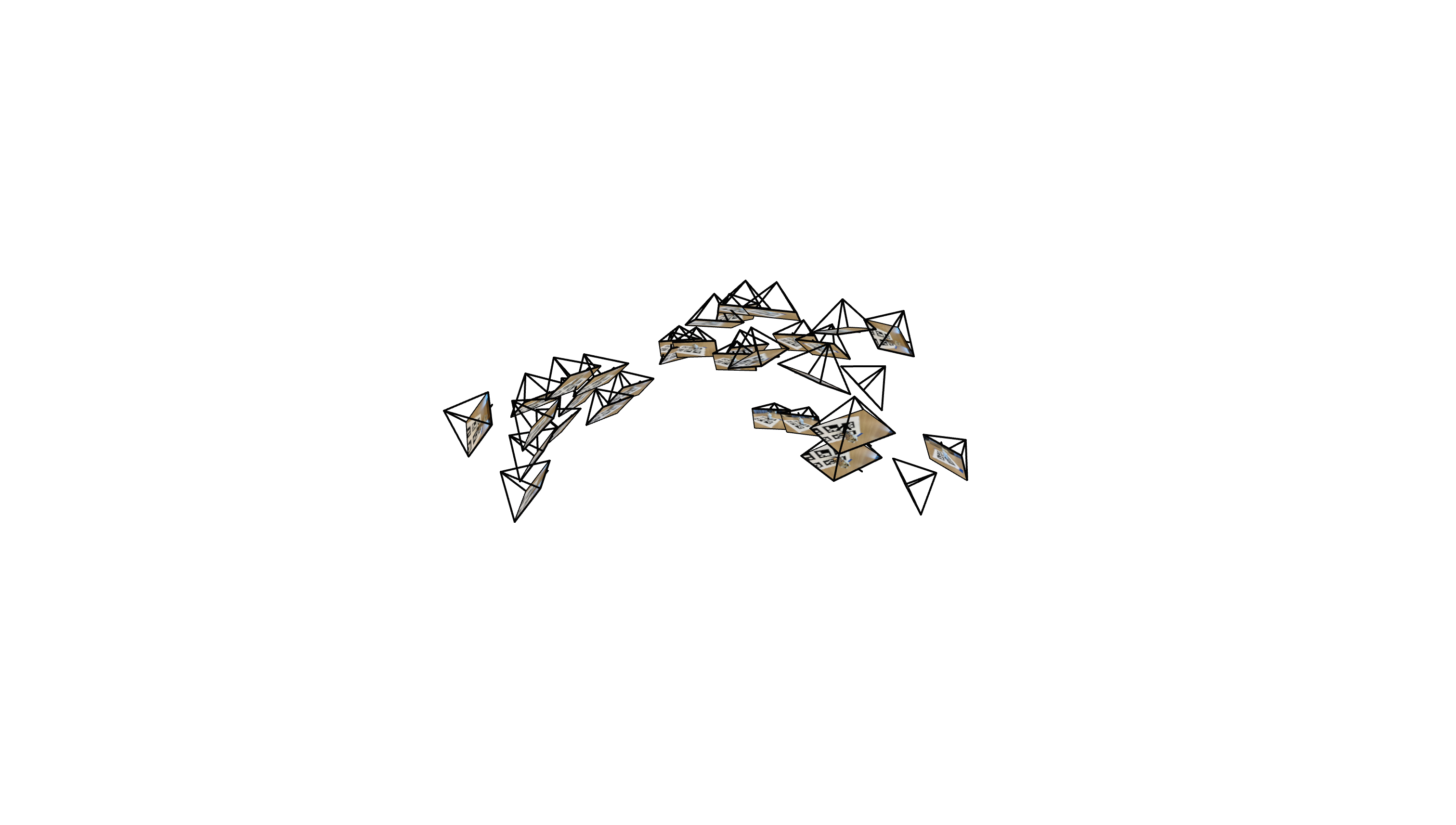
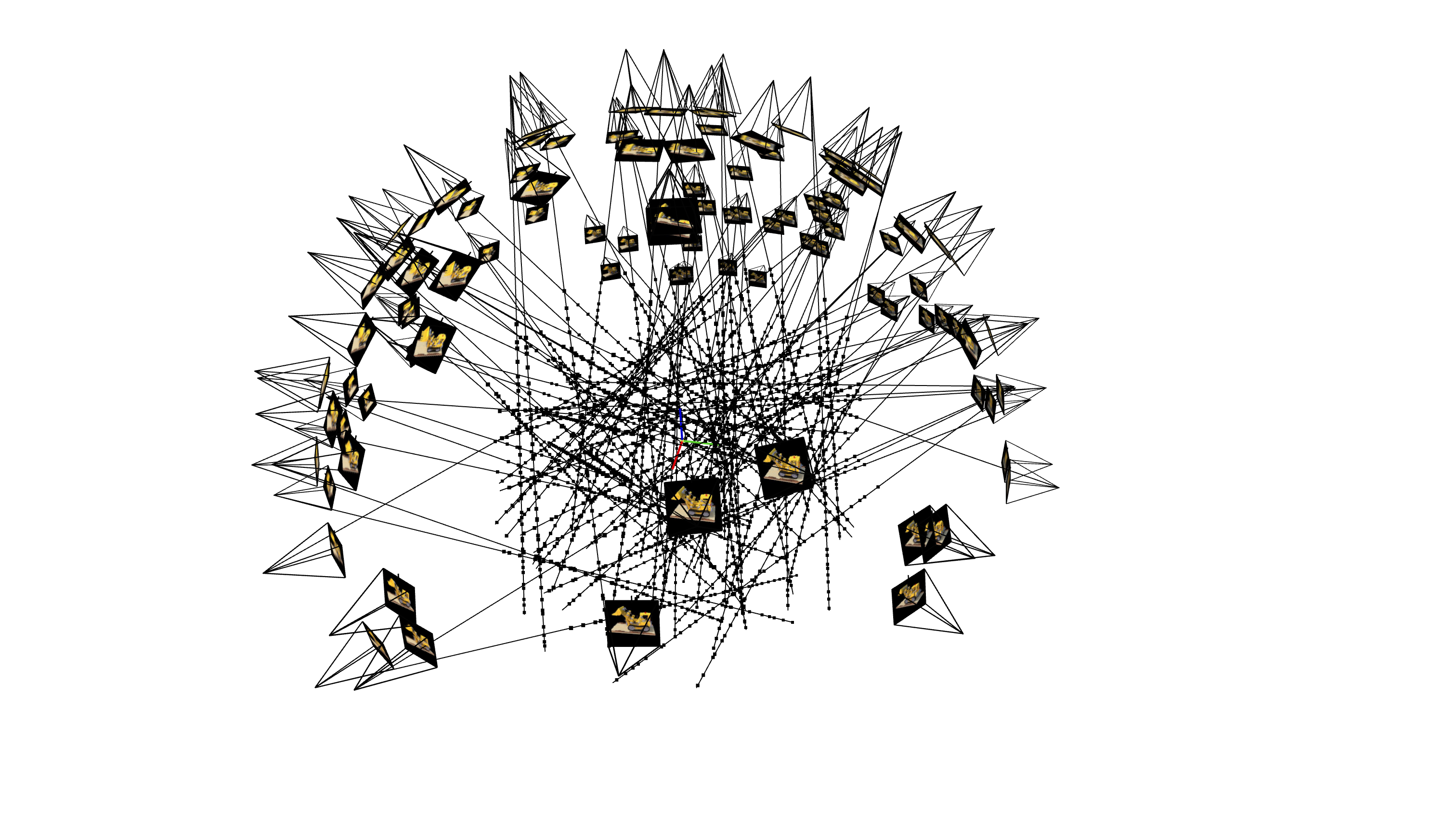
To visualize the pose estimation results, we use Viser (developed by UC Berkeley) to display camera frustums in 3D space. The visualization shows the position and orientation of each camera relative to the ArUco tag's coordinate system (which serves as the world origin).

Part 0.4: Undistorting Images and Creating a Dataset

After obtaining camera intrinsics and pose estimates, we undistort all images using cv2.undistort() to remove lens distortion, as NeRF assumes a perfect pinhole camera model. If black boundaries appear after undistortion, we use cv2.getOptimalNewCameraMatrix() to compute a new camera matrix that crops out invalid pixels, and update the principal point to account for the crop offset. Finally, we package everything into a .npz file format using np.savez() containing training/validation images, camera-to-world transformation matrices (c2ws), and focal length, ready for NeRF training.

Camera Pose Visualization

Visualization of camera frustums showing the estimated poses for the captured object scans:

Camera frustums for the ATAT walker scan showing the distribution of viewpoints around the object

Camera frustums for the Lufulu scan showing the distribution of viewpoints around the object

Part 1: Fit a Neural Field to a 2D Image

Before jumping into 3D NeRF, we first familiarize ourselves with neural fields using a 2D example. In 2D, the Neural Radiance Field becomes simply a Neural Field, where we learn a function that maps 2D pixel coordinates to RGB color values. This section creates a neural field that can represent a 2D image and optimizes it to fit the target image.

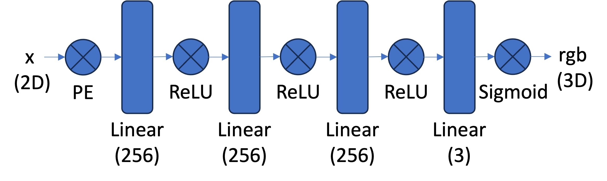
Network Architecture

The network consists of a Multilayer Perceptron (MLP) with Sinusoidal Positional Encoding (PE) that takes 2D pixel coordinates as input and outputs 3D RGB color values. The MLP is a stack of fully connected layers (torch.nn.Linear()) with non-linear activations (torch.nn.ReLU()), with a final torch.nn.Sigmoid() layer to constrain outputs to the range [0, 1] for valid pixel colors.

MLP architecture with Positional Encoding: 2D coordinates → PE → Linear(256) → ReLU → Linear(256) → ReLU → Linear(256) → ReLU → Linear(3) → Sigmoid → RGB output

Implementation Details

For training, we implement a dataloader that randomly samples pixels at each iteration to handle high-resolution images within GPU memory limits. Both coordinates (normalized by image dimensions) and colors (normalized by 255.0) are scaled to [0, 1]. We use mean squared error loss (torch.nn.MSELoss) between predicted and ground truth colors, train with Adam optimizer (torch.optim.Adam) at a learning rate of 1e-2, and run for 1000-3000 iterations with a batch size of 10k. We measure reconstruction quality using Peak Signal-to-Noise Ratio (PSNR), computed from MSE for normalized images.

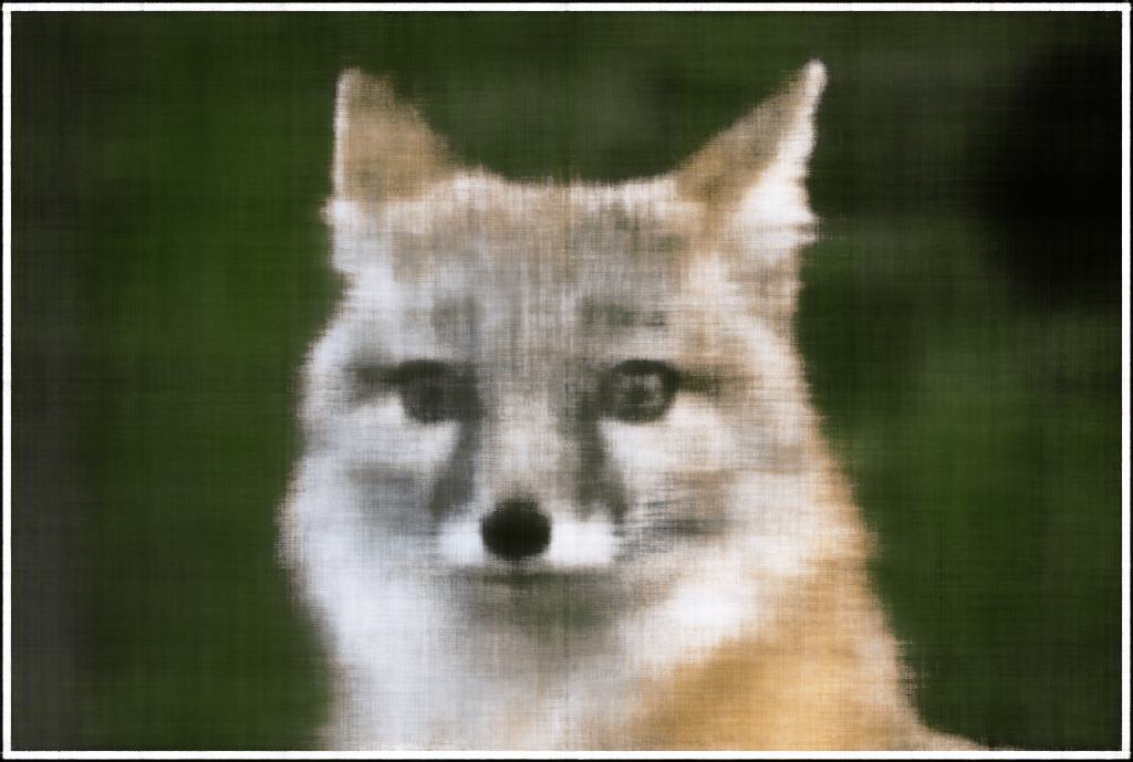
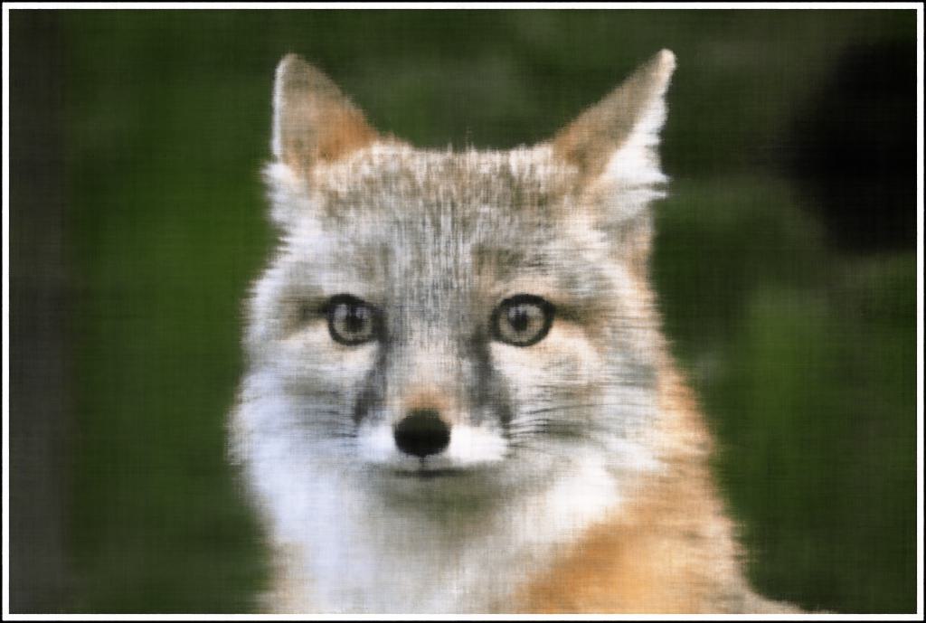
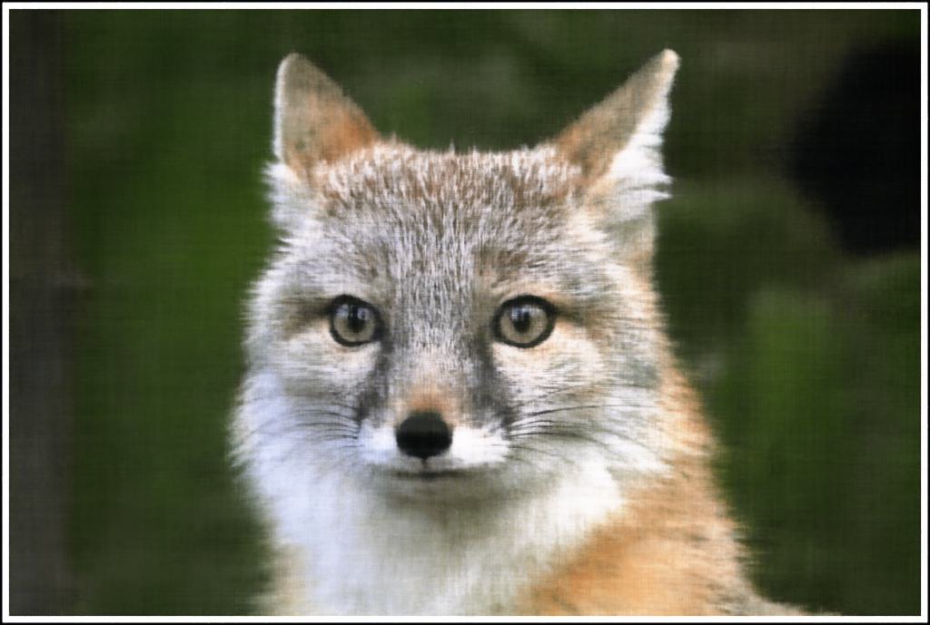
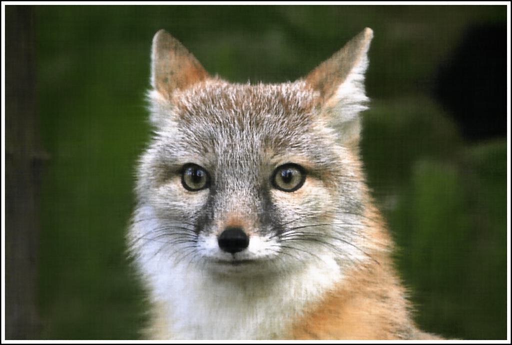
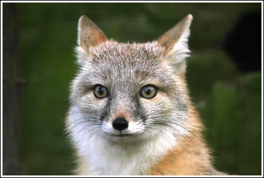
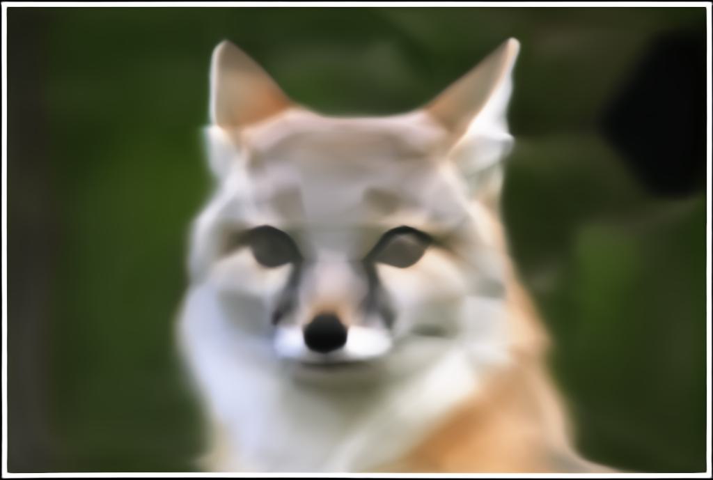
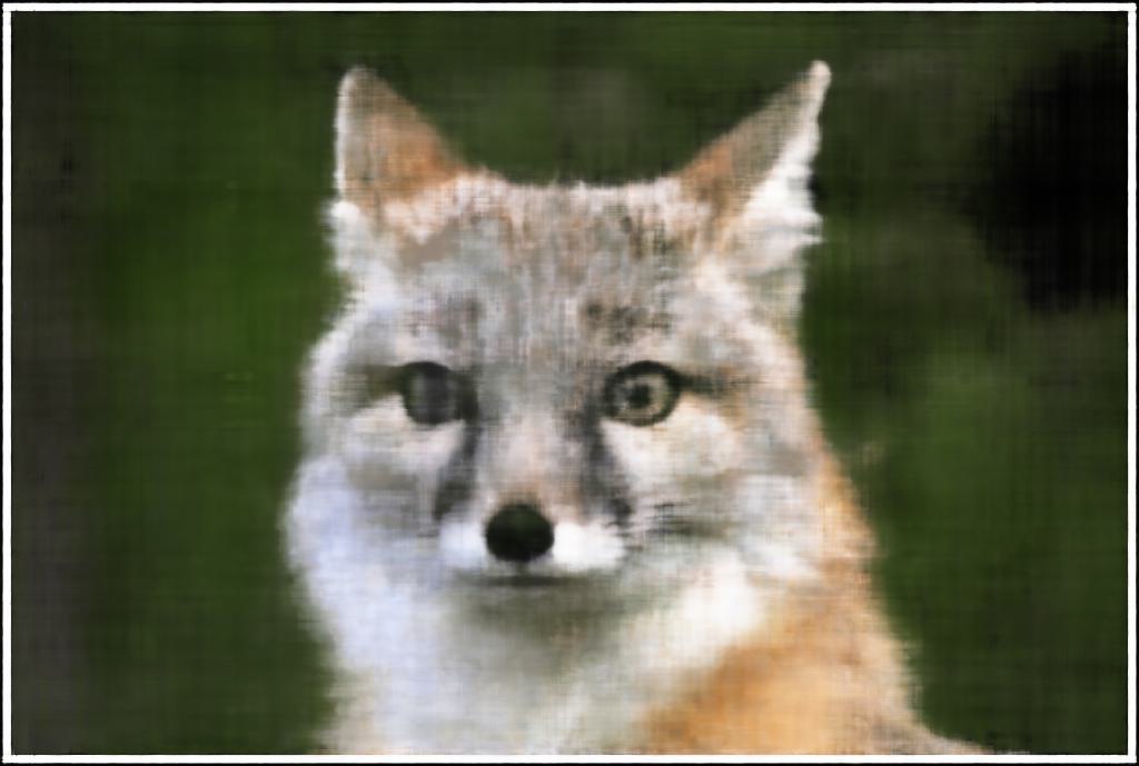
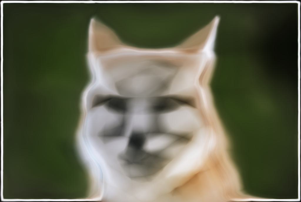
Training Progression

Below we show the training progression on two different images, demonstrating how the neural field gradually learns to represent the target image. Note that one iteration is a single gradient update of the network parameters from sampling a batch of pixels.

Fox Image Training

Iteration 100

Iteration 250

Iteration 500

Iteration 1000

Iteration 2000

Iteration 3000

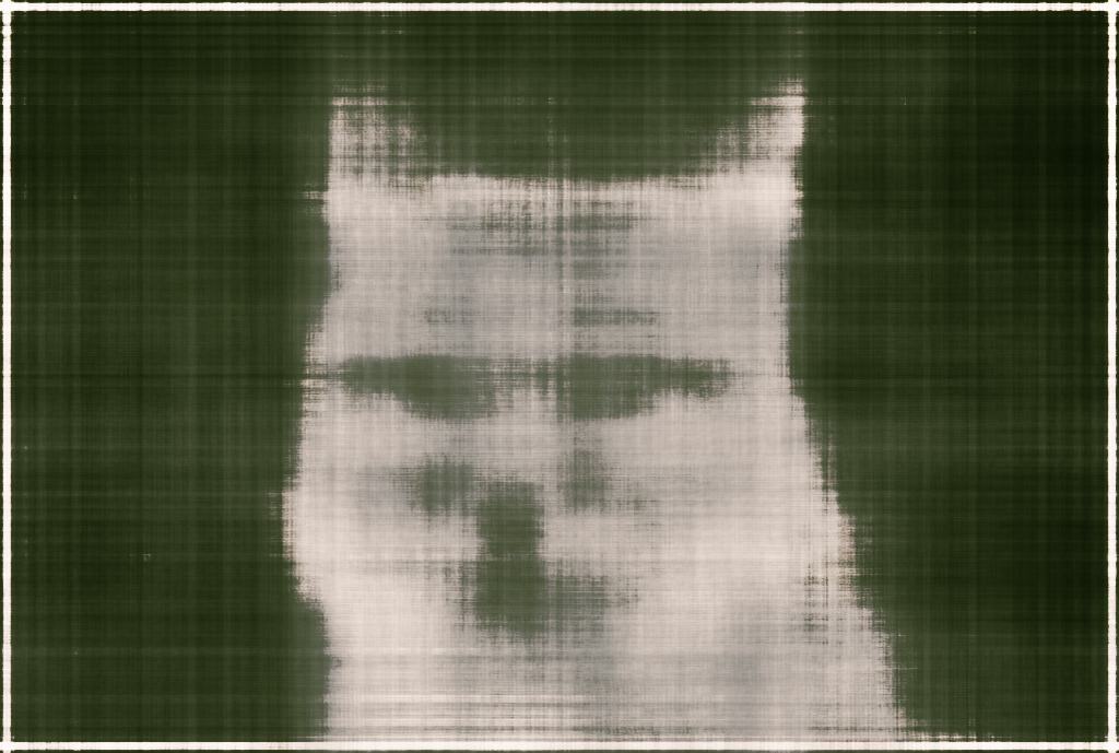
Remi Paris Image Training

Iteration 100

Iteration 250

Iteration 500

Iteration 1000

Iteration 2000

Iteration 3000

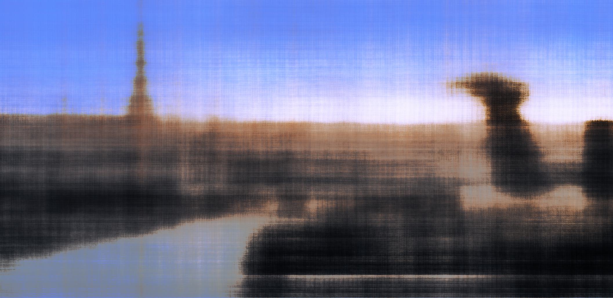
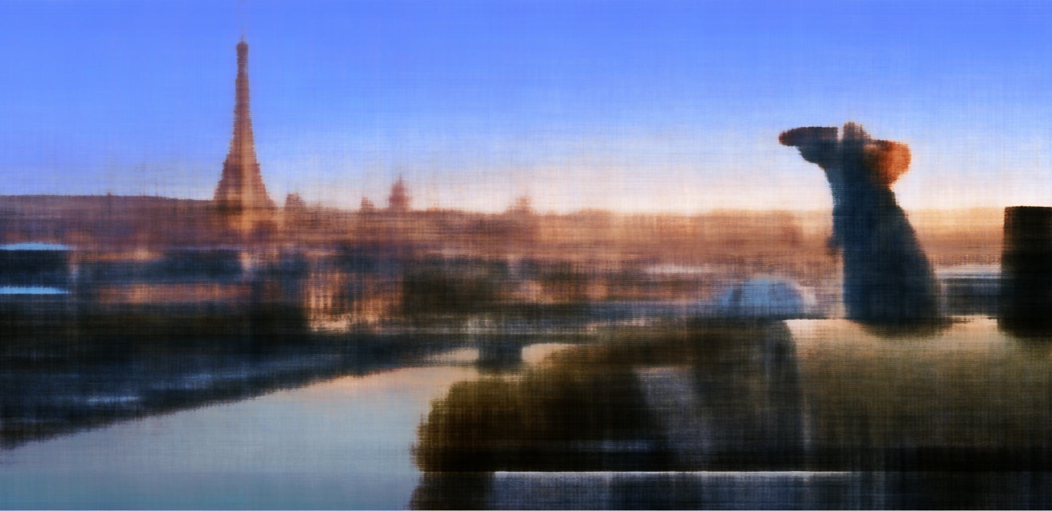
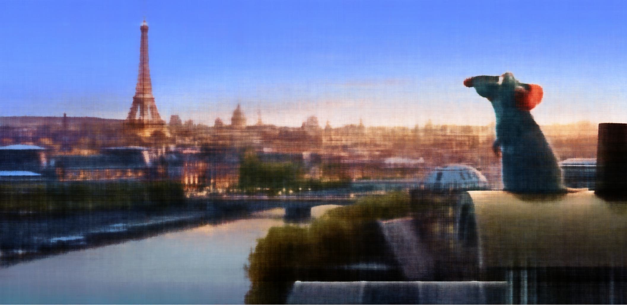
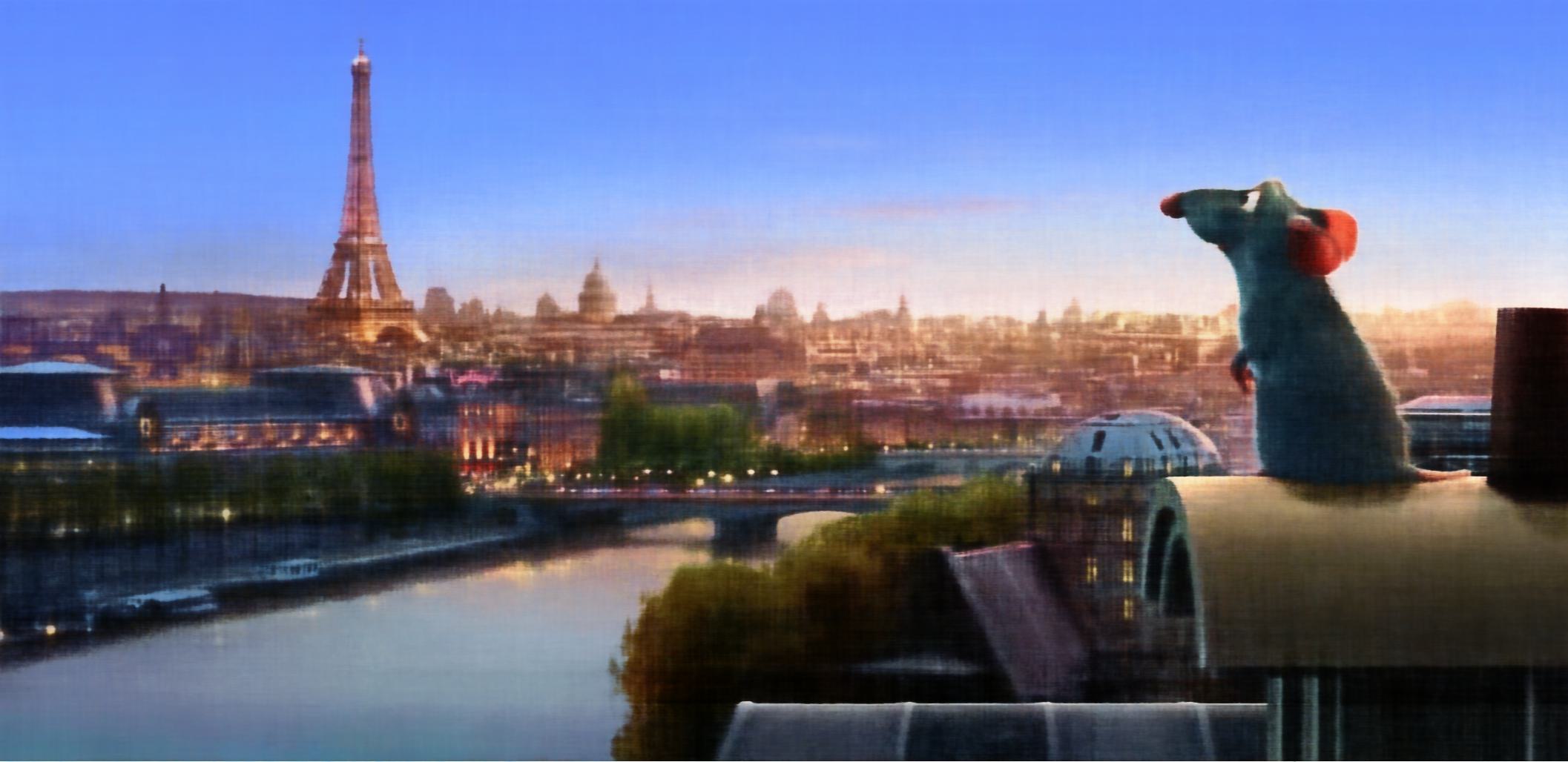
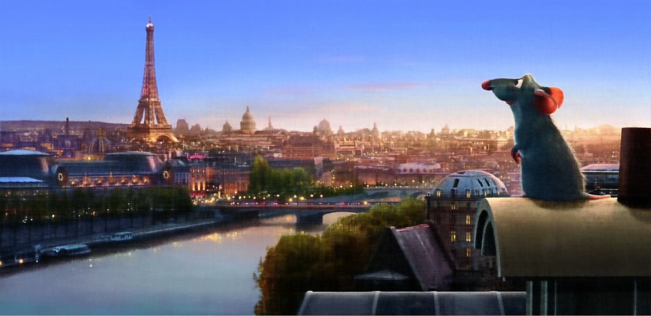
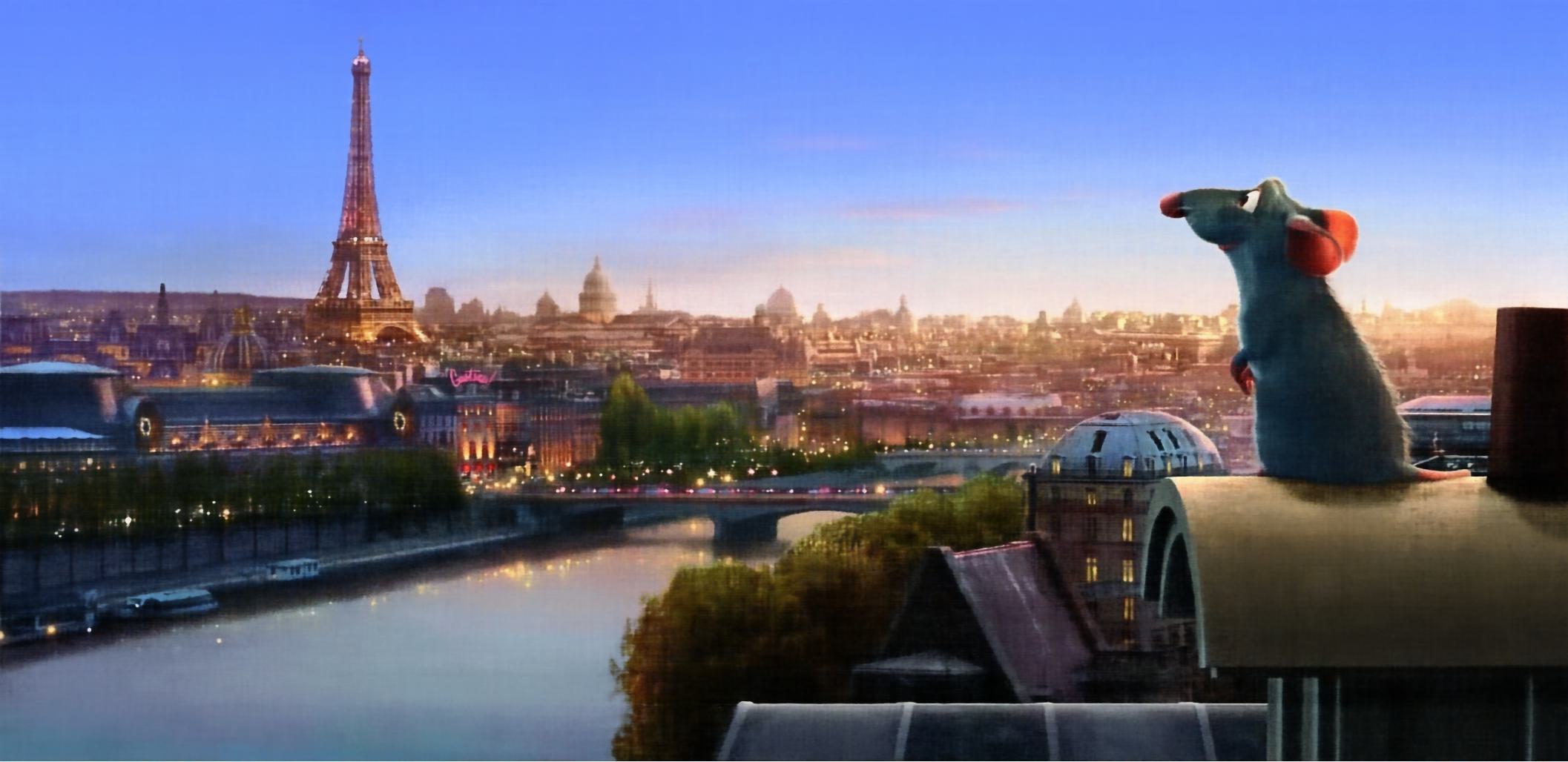
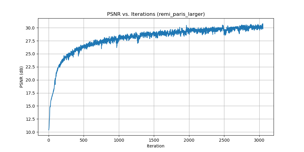
PSNR Curve for Remi Paris

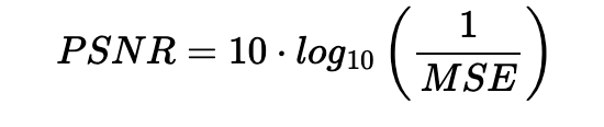
While we optimize the network by minimizing mean squared error (MSE) loss, we use Peak Signal-to-Noise Ratio (PSNR) as our evaluation metric to measure reconstruction quality. PSNR provides a more interpretable measure of image quality in decibels. The relationship between MSE and PSNR is given by:

PSNR progression during training on the Remi Paris image. The network is optimized to minimize MSE, but PSNR is used as the evaluation metric.

Hyperparameter Analysis

We explore the effects of varying the layer width (channel size) and the maximum frequency L for positional encoding. Below is a 2×2 grid showing final results (at iteration 3000) for different hyperparameter combinations, demonstrating how lower values affect the reconstruction quality.

Width=512, L=10 (baseline)

Width=512, L=2 (low frequency)

Width=64, L=10 (narrow network)

Width=64, L=2 (low capacity)

We can see that positional encoding with lower max frequency (L=2) results in the model failing to capture finer, higher frequency details in the image. In contrast, small width results in the model not being as accurate, but the effect is not as severe. This explains the importance of the PE component in NeRF as image and eventually multi view reconstruction relies on it to capture the fine details of the scene.

Part 2: Fit a Neural Radiance Field from Multi-view Images

Now that we are familiar with using a neural field to represent a 2D image, we proceed to the more interesting task of using a neural radiance field to represent a 3D space through inverse rendering from multi-view calibrated images. For this part, we use the Lego scene from the original NeRF paper, but with lower resolution images (200×200) and preprocessed cameras.

Part 2.1: Create Rays from Cameras

To render a 3D scene using NeRF, we need to cast rays from each camera through each pixel. This involves three key transformations: converting between camera and world coordinates, converting between pixel and camera coordinates, and finally constructing rays from pixel coordinates. For this, we need to define some transformations between different coordinate systems:

Camera to World Coordinate Conversion

The transformation between world space $\mathbf{x}_w$ and camera space $\mathbf{x}_c$ can be defined using a rotation matrix $\mathbf{R}$ and a translation vector $\mathbf{t}$:

Pixel to Camera Coordinate Conversion

For a pinhole camera with focal length $f$ and principal point $(c_x, c_y)$, the intrinsic matrix $\mathbf{K}$ is defined as:

Pixel to Ray

A ray can be defined by an origin vector $\mathbf{r}_o$ and a direction vector $\mathbf{r}_d$. For a pinhole camera, we need to compute these for every pixel $\mathbf{uv}$.

Part 2.2: Sampling

Once we have rays, we need to sample points along them to query the neural radiance field. This involves two steps: sampling rays from images and sampling points along each ray.

Sampling Rays from Images

Similar to Part 1, we randomly sample pixels from images to get ray origins and directions. We account for the offset from image coordinates to pixel centers by adding 0.5 to the UV pixel coordinate grid. For multiple images, we flatten all pixels from all images into a single global pool and randomly sample N rays using index math. Specifically, we compute the total number of pixels across all images, randomly permute indices, and use integer division and modulo operations to recover which image and which pixel (row, column) each sampled index corresponds to.

Sampling Points along Rays

After obtaining rays, we discretize each ray into 3D sample points. The simplest approach is to uniformly sample points along the ray:

Part 2.3: Putting the Dataloading All Together

Similar to Part 1, I implemented a dataloader that randomly samples pixels from multiview images. The key difference is that the dataloader now converts pixel coordinates into rays, returning ray origins, ray directions, and corresponding pixel colors. This combines the ray construction from Part 2.1 with the sampling strategy from Part 2.2 into a unified pipeline.

To verify the implementation, I used visualization code to plot the cameras, rays, and samples in 3D. Testing with rays sampled from a single camera first helped ensure all rays stay within the camera frustum and catch any potential bugs early.

Visualization of camera frustums, rays, and sample points in 3D space, verifying correct ray construction and sampling

Part 2.4: Neural Radiance Field

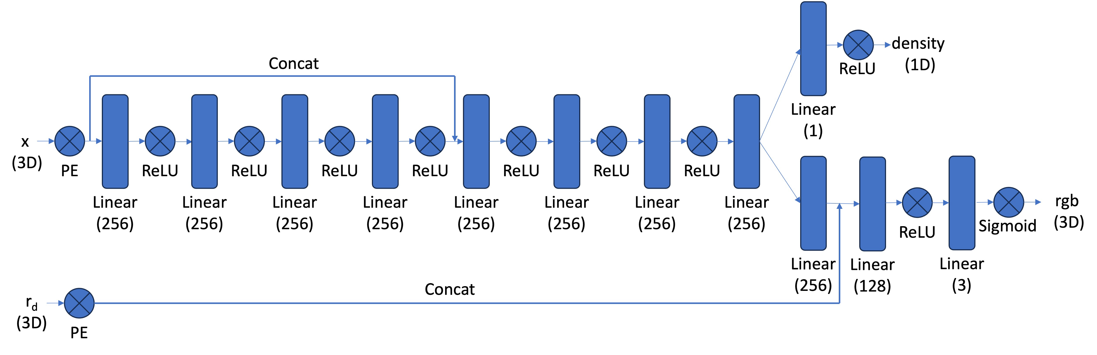
After obtaining 3D sample points along rays, we use a neural network to predict the density and color for each point. The network is similar to the MLP from Part 1, but with three important modifications:

1. Input and Output Changes: The input is now 3D world coordinates along with a 3D ray direction vector. The network outputs both color and density. Since the color of each point in a radiance field depends on the viewing direction, we condition the color prediction on the ray direction. We use Sigmoid to constrain output colors to the range (0, 1) and ReLU to ensure density values are positive. The ray direction is also encoded using positional encoding, but typically with a lower frequency (e.g., L=4) compared to the coordinate positional encoding (e.g., L=10).
2. Deeper Network: Since we're now optimizing a 3D representation instead of 2D, we need a more powerful network with more layers to capture the increased complexity.
3. Input Injection: We inject the input (after positional encoding) into the middle of the MLP through concatenation. This is a general deep learning technique that helps the network retain information about the input throughout the forward pass.

NeRF network architecture: 3D coordinates and ray direction → Positional Encoding → Deep MLP with input injection → Density and view-dependent color output

Part 2.5: Volume Rendering

Once we have sampled points along rays and queried the neural network for densities and colors at those points, we need to integrate these values along each ray to compute the final pixel color. This is done through volume rendering.

Continuous Volume Rendering Equation

The core volume rendering equation integrates contributions along the ray:

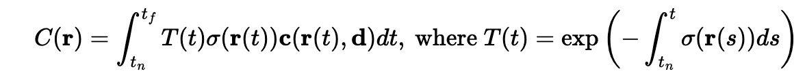
This equation means that at every small step $dt$ along the ray, we add the contribution of that small interval to the final color. The integral performs infinitely many additions of these infinitesimally small intervals. Here, $T(t)$ represents the transmittance (probability of the ray not terminating before location $t$), $\sigma(\mathbf{r}(t))$ is the density at location $\mathbf{r}(t)$, and $c(\mathbf{r}(t), \mathbf{d})$ is the color predicted by the network at that location with viewing direction $\mathbf{d}$.

Discrete Volume Rendering Approximation

For practical computation, we use a discrete approximation of the continuous integral:

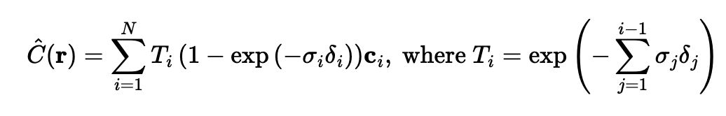
where $c_i$ is the color obtained from our network at sample location $i$, $T_i$ is the probability of a ray not terminating before sample location $i$, and $(1 - \exp(-\sigma_i \delta_i))$ is the probability of terminating at sample location $i$ (also called the alpha value or opacity).

Implementation

Our implementation computes the volume rendering in three steps:

1. Compute opacity values: For each sample, we compute $\alpha_i = 1 - \exp(-\sigma_i \delta_i)$, which represents the probability of the ray terminating at that sample.
2. Compute transmittance values: We use torch.cumsum() to efficiently compute the cumulative sum of $\sigma_i \delta_i$ values along each ray. This cumulative sum is then shifted and padded with zero to model the "up to but not including" effect for transmittance, and finally exponentiated to get $T_i = \exp(-\sum_{j=1}^{i-1} \sigma_j \delta_j)$.
3. Weighted sum: The final rendered color is computed as a weighted sum: $\hat{C}(\mathbf{r}) = \sum_{i=1}^{N} T_i \alpha_i c_i$, where each color is weighted by both its transmittance and opacity.

The use of torch.cumsum() allows us to efficiently compute all transmittance values in parallel for all rays and all samples, making the implementation both correct and computationally efficient.

Results

We trained the NeRF model on the Lego dataset and evaluated its performance on novel view synthesis. Below we show the training progression and final results.

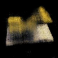
Training Progression

The following images show how the NeRF model improves over training iterations, gradually learning to represent the 3D structure and appearance of the Lego scene:

Iteration 200

Iteration 500

Iteration 800

Iteration 1200

Iteration 1500

Final Results

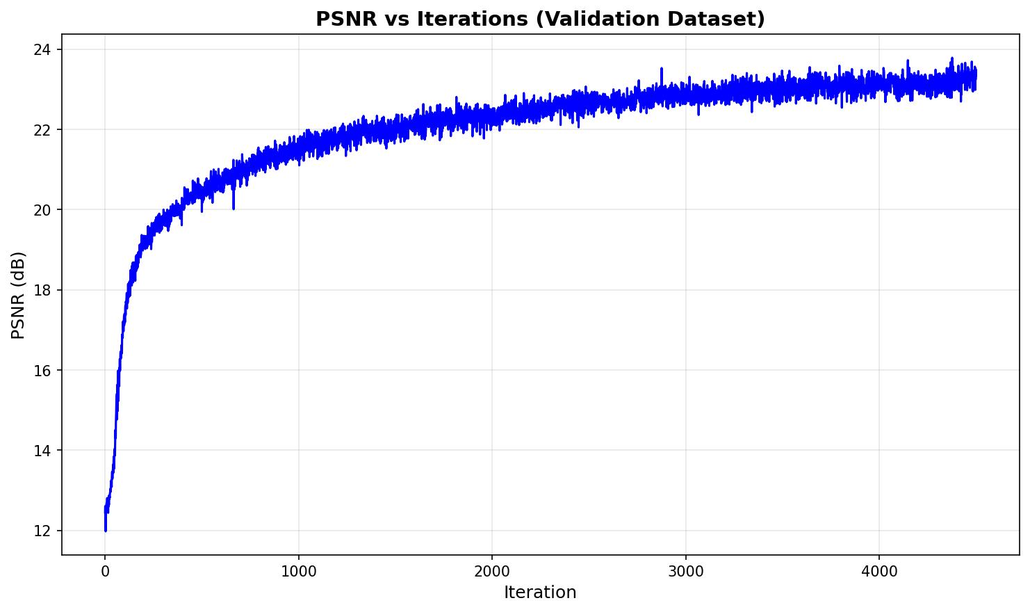
After training for 4500 iterations, the NeRF model achieves high-quality novel view synthesis. We evaluate the model on the validation set (images not seen during training) to measure generalization performance.

Validation Set PSNR

The Peak Signal-to-Noise Ratio (PSNR) on the validation set measures how well the model generalizes to unseen viewpoints. Higher PSNR values indicate better reconstruction quality:

PSNR progression on the validation set during training. The model is evaluated on images not seen during training to measure generalization performance.

Novel View Synthesis

The trained NeRF model can render the scene from any viewpoint, including novel camera positions not present in the training data. Below is a spherical render showing the model's ability to synthesize views from a complete 360-degree rotation:

Spherical render of the Lego scene, demonstrating the model's ability to synthesize novel views from any camera angle

Part 2.6: Training with Your Own Data

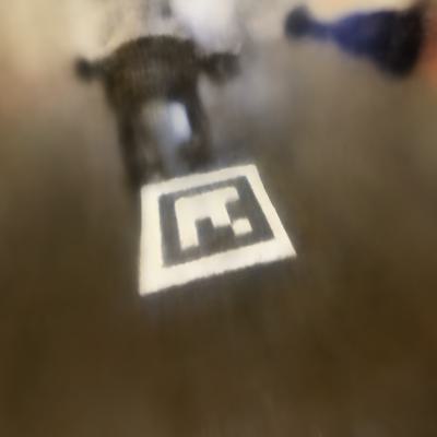
Using the dataset created in Part 0, I trained a NeRF model on my custom object: an ATAT walker from Star Wars. The same pipeline used for the Lego dataset was applied to the ATAT walker images captured during the 3D scanning process.

After training the NeRF on the custom dataset, I rendered novel views from the scene to demonstrate the model's ability to synthesize new viewpoints of the ATAT walker. The trained model successfully captures the geometric structure and appearance of the object, allowing for realistic rendering from any camera angle.

Hyperparameter Tuning

For training the ATAT walker NeRF, the key hyperparameters that needed adjustment were the near and far bounds for ray sampling. These parameters define the depth range along each camera ray where we sample 3D points. The near parameter specifies the closest distance from the camera where we start sampling, while far specifies the farthest distance. These bounds are crucial because they determine which portion of 3D space the network learns to represent—if the bounds are too narrow, we might miss parts of the object, and if they're too wide, we waste computational resources on empty space.

For the ATAT walker dataset, I adjusted these bounds based on the actual distance and scale of the object relative to the camera positions. I used near = 0.0213 and far = 0.2754, which are significantly smaller than the Lego scene values (near=2.0, far=6.0) due to the different scale and camera-to-object distance in my custom dataset. The other hyperparameters (network architecture, positional encoding frequency, learning rate, number of samples per ray) were kept the same as those used for the Lego NeRF to maintain consistency and leverage the same proven configuration.

Results

Below we show the training progression, metrics, and results for the ATAT walker NeRF model.

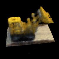
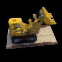
Training Progression

The following images show how the NeRF model improves over training iterations, gradually learning to represent the 3D structure and appearance of the ATAT walker scene:

Iteration 1000

Iteration 2000

Iteration 3000

Iteration 4000

Iteration 5000

Iteration 6000

Iteration 7000

Iteration 8000

Iteration 9000

Iteration 10000

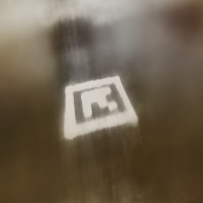
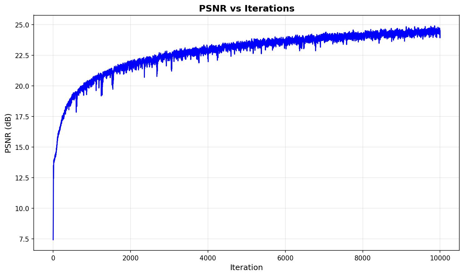
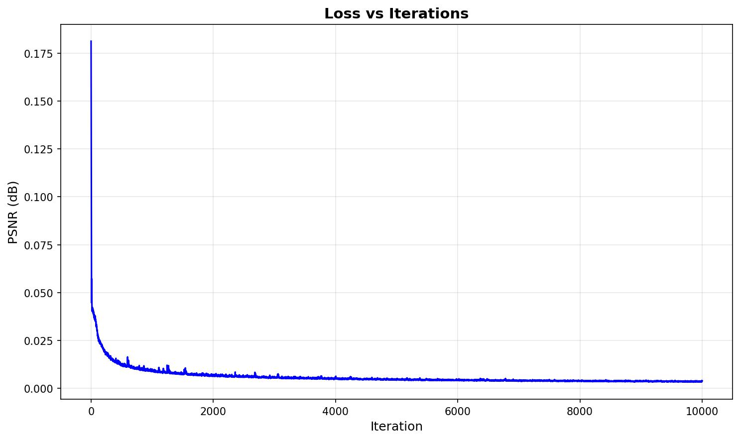
Training Metrics

The following plots show the PSNR and loss curves during training of the ATAT walker NeRF model:

PSNR progression during training on the ATAT walker dataset

Training loss progression during training on the ATAT walker dataset

Novel View Synthesis

The trained NeRF model can render the ATAT walker scene from any viewpoint, including novel camera positions not present in the training data. Below are spherical renders showing the model's ability to synthesize views from complete 360-degree rotations:

Spherical render of the ATAT walker scene

Alternative spherical render of the ATAT walker scene

Conclusion

This project successfully implemented a complete Neural Radiance Fields (NeRF) pipeline, from camera calibration and 3D object scanning to training neural networks for novel view synthesis. The project demonstrated the power of neural fields, first in 2D image representation and then extended to 3D scene reconstruction from multi-view images.

Through careful implementation of camera pose estimation, ray construction, volume rendering, and neural network optimization, we achieved high-quality novel view synthesis on both synthetic (Lego) and real-world (ATAT walker) datasets. The results showcase how neural radiance fields can capture complex 3D geometry and view-dependent appearance, enabling realistic rendering from any camera angle. The project highlights the importance of proper camera calibration, positional encoding, and volume rendering techniques in creating photorealistic 3D scene representations.